Solving Transient Models That Have Inconsistent Initial Values
When solving a transient (i.e., time-dependent) study in COMSOL Multiphysics®, it is important to have your model set up so that the initial conditions are consistent with the loads and boundary conditions. This is important for any time-dependent model, but it is especially notable when performing transient fluid flow studies. In this article, we will explain why such consistency is important, its impact on your model, and the different approaches that you can use to solve the transient model equations when you have inconsistent initial values.
Background
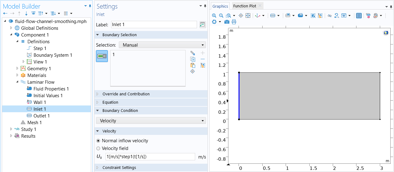
To illustrate with context why it is necessary for the initial values of your model to be consistent with the loads and boundary conditions, let us use an example. A simple fluid flow model is represented below, consisting of a 2D channel that is 3 meters long and 1 meter wide, where the left boundary is the inlet and the right boundary is the outlet. We want to solve for the laminar flow of a fluid through a channel. The fluid has a density of 1 kg/m3 and a viscosity of 0.01 Pa·s. A velocity of 1 m/s is specified at the inlet, and a zero-pressure boundary condition is applied to the outlet.
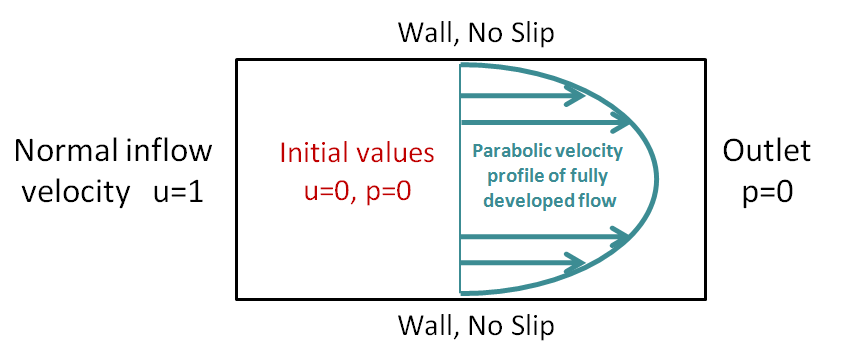 A diagram of the fluid flow example model.
These boundary conditions lead to a mismatch between the value of the velocity at the inlet (u = 1 m/s) and the initial value of the velocity (u = 0 m/s) in the channel. This is referred to as inconsistent initial values.
 A screenshot of the COMSOL Multiphysics UI showing the settings for the sample model's Inlet boundary condition.
The model setup for our example in the software, with the settings for the Inlet boundary condition displayed.
A screenshot of the COMSOL Multiphysics UI showing the settings for the sample model's Inlet boundary condition.
The model setup for our example in the software, with the settings for the Inlet boundary condition displayed.
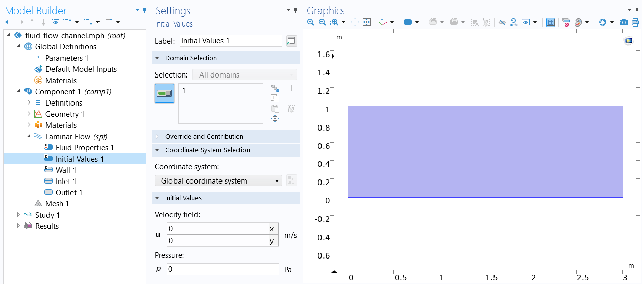 A screenshot of the COMSOL Multiphysics UI showing the default settings for the Initial Values node.
The default Initial Values node with the default settings.
A screenshot of the COMSOL Multiphysics UI showing the default settings for the Initial Values node.
The default Initial Values node with the default settings.
When your model has inconsistent initial values, you may observe the solver taking very small time steps or ending the computation and reporting an error message like the following:
Failed to find consistent initial values.
Last time step is not converged.
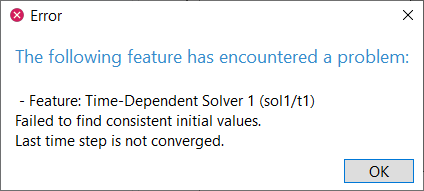
An error message stating the source of the error that prohibited the model computation from completing.
The COMSOL Multiphysics® software will, by default, attempt to reconcile inconsistent initial values by taking a small time step that is a fraction of the initial time step using a backward Euler method. The initial time step is by default determined based on the total simulation time span. However, it is also possible to specify the initial time step and change the fraction of the initial step used by the backward Euler method — a backward differentiation formula (BDF) method — for the consistent initialization. These settings will affect the results of the consistent initialization procedure.
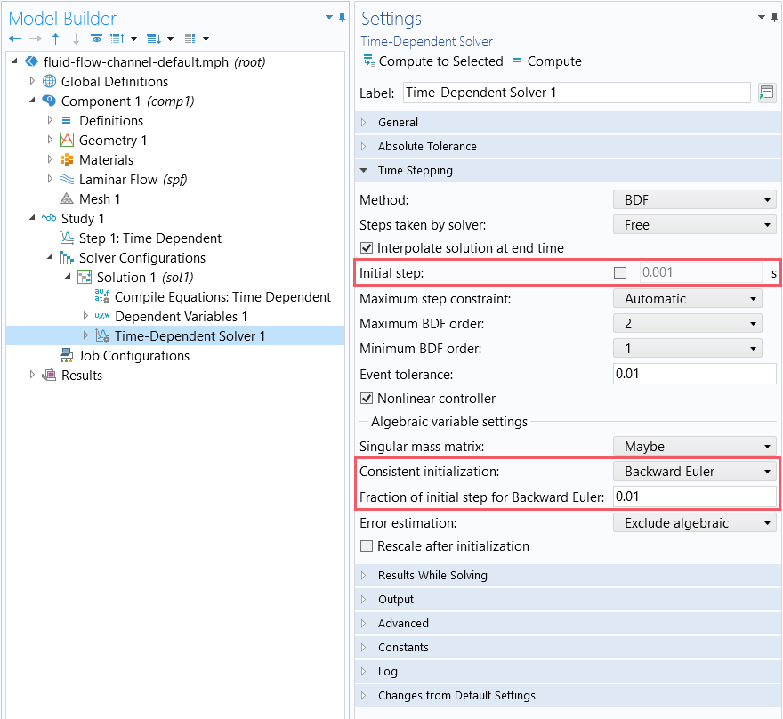
The Settings window showing the default settings for the Time-Dependent Solver.
The consistent initialization may fail if the backward Euler step is too large or if the boundary conditions in your model are inconsistent with each other or the physics in your model. More commonly, the results may be very far from what is expected, and the solver will likely need to take very small time steps at the beginning of the simulation to evolve from the initial solution. This is undesirable because it can lead to long solution times.
In many cases this consistent initialization is not strictly needed, and it might be better to turn it off to ensure that your model smoothly ramps up all loads and boundary conditions from consistent initial values. In this article, we will present you with two ways to do so. The approaches we recommend for computing transient models with inconsistent initial values are the following:
- Initialize the time-dependent study with a Stationary study step
- Ramp up the boundary conditions over time
Please note that if your boundary conditions are truly inconsistent, then the resolutions in this article will not be applicable. Always check the applied loads and boundary conditions in your model carefully for consistency. The recommendations we outline here are only applicable to well-posed problems, so it is important that your model meet that threshold first.
Approach 1: Initializing Time-Dependent Studies with Stationary Studies
The first approach you can use to solve a time-dependent model with inconsistent initial values is to initialize your transient study with a stationary study. There are a couple of ways that this can be done, as are described below.
Using Multiple Steps
A single study can include multiple study steps. By default, the results of each study step are passed on to the following study step as its initial values. When a Stationary study step is added before a Time Dependent study step, the study will solve first for the fields under the steady-state assumption and then use these computations to provide consistent initial values for the transient step, overriding the initial values specified within the Initial Values node in the physics interface. As long as the two steps are within the same study, as shown in the screenshot below, no other changes are needed. When the study is solved, both steps will be recomputed.
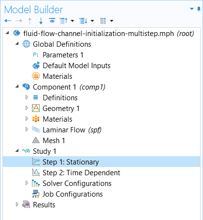
A Stationary study step is used to compute the initial values for the transient study step.
You can see this multistep approach firsthand in the attached model file for the fluid flow example introduced earlier.
Using Multiple Studies
Values of Dependent Variables Settings Section
It is also possible to split the analysis into two separate studies. In this way, the Stationary study step and the Time Dependent study step are each added under two different studies. This setup requires that the Values of Dependent Variables section in the settings for the Time Dependent study step are set to refer to the results of the stationary study, as shown in the screenshot below.
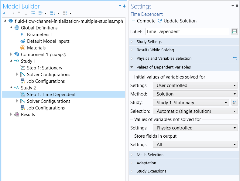
The settings for the Time Dependent study step node, which uses the initial values computed from the previous stationary study.
You can explore how this version of the approach was implemented for the fluid flow example in the model file included here.
Although this strategy is available, it does come with a number of drawbacks:
- First, depending on the problem you are modeling, a stationary solution might not exist. This is particularly common for fluid flow models near the onset of turbulence, where steady boundary conditions result in an unsteady (time-varying) flow field. It can also be the case that a steady-state solution for your model is numerically difficult to find. Please see our resource discussing how to improve the convergence of nonlinear, stationary models to learn how to address such cases.
- Second, the objective of the transient model may be to investigate the startup behavior as the system evolves from the at-rest state.
In either case, use the second method, described below.
Using the withsol Operator
When splitting the analysis into two separate studies, another option for referring to the results of the stationary study would be to use the withsol operator. The withsol operator enables you to extract and use the solution from one study as input for another study. It is equivalent to making the changes in the Values of Dependent Variables section of a study step's settings, discussed in the preceding section.
In the Initial Values node, we can enter the appropriate syntax for using the withsol operator, formatted as: withsol('tag',expr). For a split-study analysis, where 'tag' is, we enter 'sol1' to refer to the stationary study's solver sequence, and for expr, we enter the appropriate physics variable (u for the x-component of the fluid flow velocity field, v for the y-component of the fluid flow velocity field, or p for the pressure).
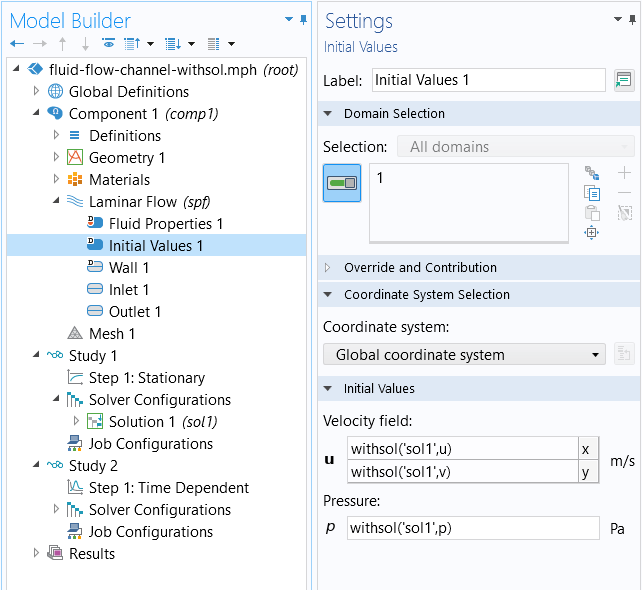
The settings for the Initial Values node, wherein the withsol _operator is used to refer to the solution for the stationary study.
More details and examples of using the withsol operator are available in our Learning Center article on this topic.
Approach 2: Ramping Up Boundary Conditions over Time
The second approach you can use to compute a time-dependent model with inconsistent initial values is to ramp up the loads and boundary conditions in your model over time.
The loads and boundary conditions in a transient model can be ramped up from values that are consistent with the initial values. The most common case is an at-equilibrium system, where the initial values are zero everywhere. The COMSOL Multiphysics® software includes several built-in functions that you can use to transition from these initial values to other values. In this example, we use the built-in Step function with smoothing, as shown in the screenshot below.
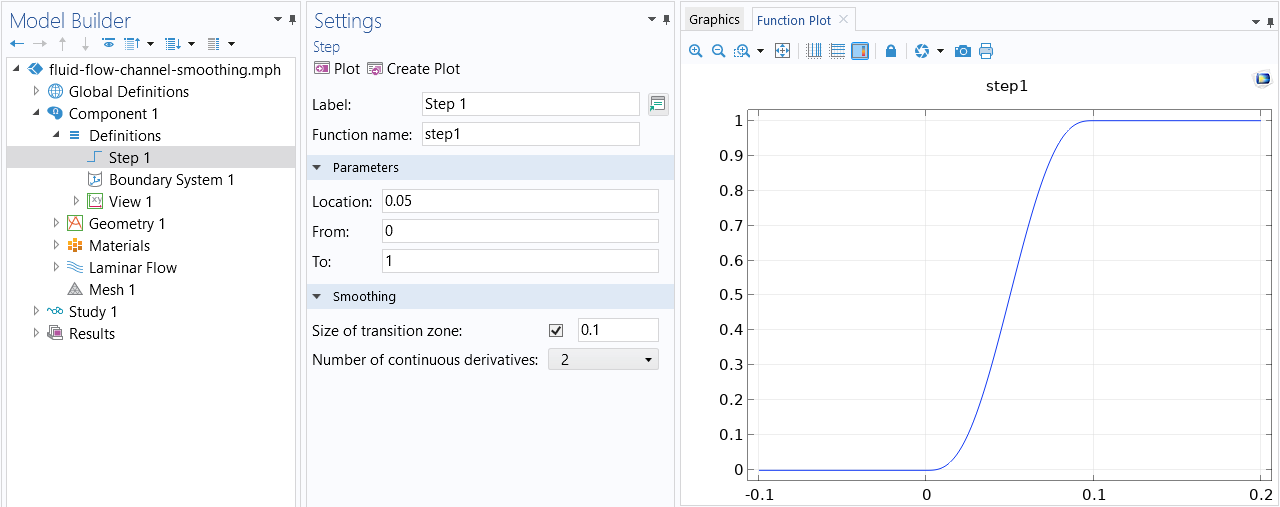 A screenshot of the COMSOL Multiphysics UI showing the Step function settings with smoothing and a function plot that shows the ramp up from the initial values.
The settings of the Step function with smoothing.
There are several other functions that also include a Smoothing option, as described here, where we discuss the modeling of step transitions. By default, these will all have a time derivative equal to zero at the start of the smoothing zone, which is helpful because there will be no abrupt step or change and it allows for a gradual transition.
We can use the smoothed Step function to modify the loads and boundary conditions of our transient fluid flow model, as shown in the screenshot below. The corresponding model file can be downloaded here.
 A screenshot of the COMSOL Multiphysics UI showing the Settings window and a function plot of the smoothed Step function.
The smoothed Step function is used to ramp up the boundary condition.
In the study for your model, you will need to choose a time span for the smoothing that is physically realistic for the problem at hand. However, instead of using a smoothing that is physically realistic, it may be reasonable to introduce a very gradual ramping, since this may solve more easily.
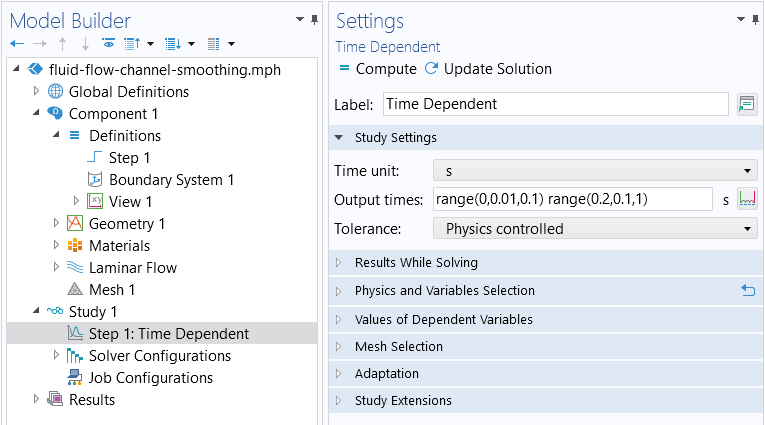
The settings for the Time Dependent study step. A short time range (from 0 to 0.1 seconds) with a smaller step size (0.01 seconds) is used where our Step function is defined and ramping up the velocity at the Inlet boundary condition in the model.
Note that not all problems will require this type of smoothing. Some problems, particularly heat transfer problems that do not involve convection, can be solved with step changes to the loads. If these step changes happen during the simulation time span, you should use the Events interface to accurately model these cases, as described here, where we discuss solving models with pulsed loads in time.
Further Learning
Using either of the above techniques to solve transient models with inconsistent initial values should resolve the issue of finding a consistent initialization, and you should not have to alter the study settings in your model. However, if you find that you still are encountering issues with convergence, this could be due to a few reasons:
- The model is not meshed finely enough. In this case, you should consider a mesh refinement study, which you can learn about here.
- The model is highly nonlinear. In this case, you should consider changing the solver configuration settings, which you can learn about here.
请提交与此页面相关的反馈,或点击此处联系技术支持。