Optimizing Multiple Parameters and Understanding Optimization Solvers
In Part 5 of this course on optimization, we begin by briefly summarizing the two model examples completed in Part 4. We then introduce the Optimal Cooling of a Tubular Reactor tutorial model, which will serve as our new guided tutorial example. The model is an example of a multiphysics optimization problem, of which the physics include heat transfer in fluids, species transport, and chemistry. The objective is to maximize the concentration of the main product species in the product stream by adjusting the temperature. We encourage you to open the software and follow along as we demonstrate how to formulate and solve this optimization problem a few different ways.
In addition, we show how to perform optimization in combination with a parametric sweep in a single study.
After completing the demonstration, we highlight several optimization tutorial models for different application areas. We then move into an in-depth discussion on optimization solvers, the different categorizations of solver methods, the differences between algorithms, what gradients are, and why and how one solver would be better than another depending on the problem. We outline how we go from the initial design to the optimal point and provide an understanding of what conditions you should use certain solvers for, particularly gradient-free solvers versus gradient-based solvers. To conclude, we showcase the Optimization Tutorials app. We recommend running the app and following along with us as we use it to perform various optimization analyses.
请提交与此页面相关的反馈,或点击此处联系技术支持。

