More on Deep Neural Network Activation Functions
Continuing the discussion on deep neural networks (DNN) from Part 1, here we will cover activation functions in more detail. Activation functions introduce nonlinearities in deep neural networks, which enables the network to learn and represent complex patterns in the data. Without activation functions, a DNN would behave as a linear model regardless of the number of layers, limiting its capacity to solve complex tasks. Different activation functions influence the learning dynamics and performance of the network by affecting the gradient flow during network optimization, impacting convergence speed and the ability to avoid issues like vanishing or exploding gradients. The choice of activation function can significantly affect the network's ability to generalize as well as its overall accuracy.
Deep Neural Network Activation Function Options
An activation function in a DNN defines how the weighted sum of the input is transformed into an output from a node or nodes in a layer of the network.
The available activation functions are Linear, ReLU (Rectified Linear Unit), ELU (Exponential Linear Unit), Sigmoid, tanh, Softplus, LeakyReLU, and GELU. Each layer can have a different activation function.
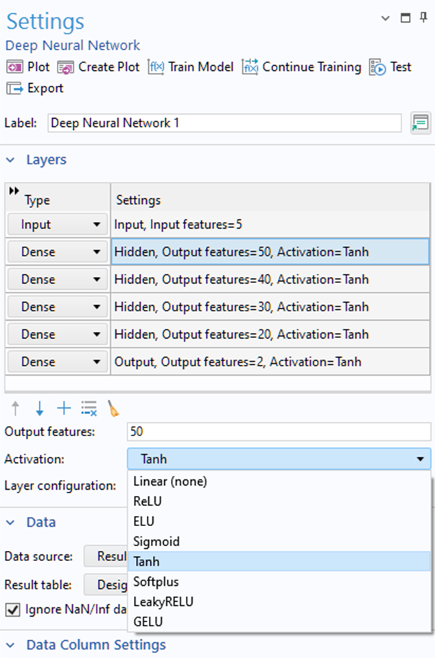
The different activation function options.
The nonlinear activation functions are designed to represent general nonlinear behavior. For example, they can represent saturation effects, which is something that, for instance, a polynomial function cannot represent. The following table describes the properties of each activation function.
| Activation Function | Expression | Graph | Properties |
|---|---|---|---|
| Linear |  |
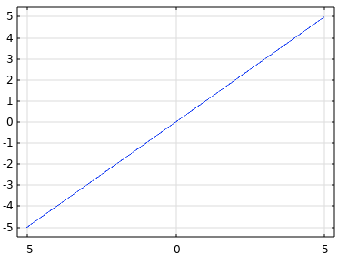 |
The Linear activation function is also sometimes referred to as no activation function. Its outputs are unbounded:  . . |
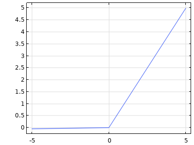
| ReLU |  |
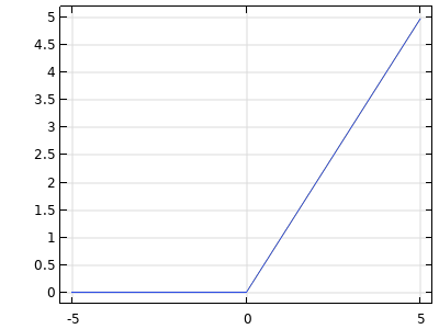 |
The ReLU activation function is piecewise linear: zero for negative values and linear for positive values. The ReLU activation function generates networks that are sometimes easier to train than other activation functions. Its outputs are unbounded:  . . |
| ELU |   |
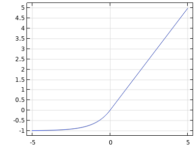 |
The ELU activation function is similar to the ReLU activation function but is smoother and more computationally intensive. Its outputs are unbounded: . |
| Sigmoid |  |
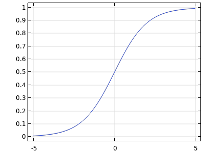 |
The Sigmoid activation function is smoothly nonlinear and s-shaped. This activation function is mostly used for probabilities and classification. Its outputs are bounded:  . . |
| tanh |   |
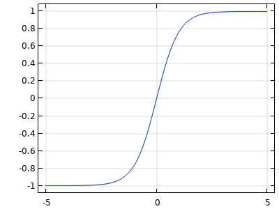 |
The tanh activation function is smoothly nonlinear and s-shaped. It is zero-centered and symmetric. Its outputs are bounded:  . This is the default option. . This is the default option. |
| softplus |  |
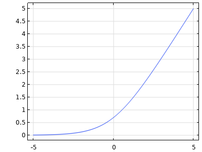 |
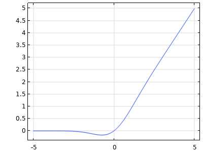
The Softplus activation function is a smooth approximation of ReLU that is always differentiable, positive, and unbounded. It is useful when smoother behavior is preferred over the hard kink of ReLU. |
| LeakyReLU |  |
 |
The LeakyReLU activation function is a variant of ReLU that uses a small nonzero slope for negative inputs and a linear response for positive inputs. It is unbounded above and allows negative outputs, which helps reduce the dying ReLU problem by maintaining a small gradient for negative values. |
| GELU |  |
 |
The GELU activation function is a smooth nonlinear activation that weights inputs by their magnitude. It is often used in modern deep learning models and provides a smoother alternative to ReLU. It is defined for all real inputs, with unbounded outputs that may be positive or negative. |
An Analytical Expression for a Deep Neural Network Model
In principle, one can use the general-purpose parameter estimation solvers in COMSOL Multiphysics® to optimize the biases and weights of a neural network. However, this is not efficient, and in practice, it is necessary to instead use the specialized Deep Neural Network function feature and the Adam optimizer. Despite this, it can be instructive to see how such an expression would look like, at least for a small network. For the  network model used for the thermal actuator, with tanh activation functions, there are 25 network parameters, and the corresponding DNN function looks like this:
dnn(x1,x2)=tanh(w3_11*(tanh(w2_11*(tanh(w1_11*(x1)+w1_21*(x2)+b1_1))+w2_21*(tanh(w1_12*(x1)+w1_22*(x2)+b1_2))+w2_31*(tanh(w1_13*(x1)+w1_23*(x2)+b1_3))+w2_41*(tanh(w1_14*(x1)+w1_24*(x2)+b1_4))+b2_1))+w3_21*(tanh(w2_12*(tanh(w1_11*(x1)+w1_21*(x2)+b1_1))+w2_22*(tanh(w1_12*(x1)+w1_22*(x2)+b1_2))+w2_32*(tanh(w1_13*(x1)+w1_23*(x2)+b1_3))+w2_42*(tanh(w1_14*(x1)+w1_24*(x2)+b1_4))+b2_2))+b3_1)
In this expression, the variables w1_11, w1_12, etc., are the network weights and the variables b1_1, b1_2, etc., are the network biases. The figure below shows the network represented as a graph, with the biases and some of the weights shown:
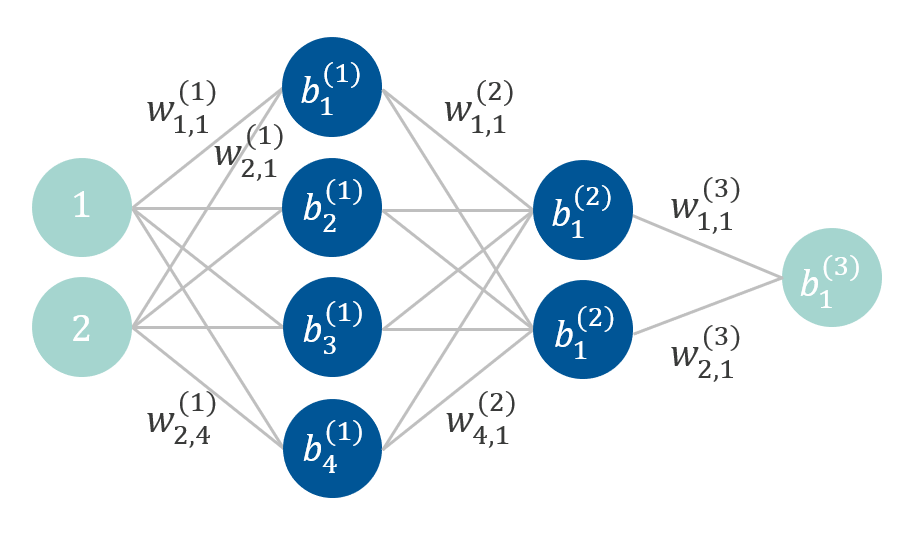
The neural network architecture for the thermal actuator model.
Their optimized values are listed in the table below and are based on scaled input data. The data needs to be scaled before the network can be optimized, since the network uses the tanh activation function, and the output values of tanh are limited to . This is a very small network, and it is easy to see that for a larger, but still small, network, such as a  , having 4321 network parameters, managing this type of expression is not practical. In the COMSOL implementation, such expressions are never explicitly formed, but the network evaluations are handled at a lower level. In addition, the scaling before and after the computation is handled automatically.
| w1_11 | w1_12 | w1_13 | w1_14 |
|---|---|---|---|
| 6.479052 | -83.5153 | -740.349 | 1028.273 |
| w1_21 | w1_22 | w1_23 | w1_24 |
| -0.01446 | -2.50149 | 0.217145 | -0.23627 |
| b1_1 | b1_2 | b1_3 | b1_4 |
| -0.03275 | 9.940952 | -2.92705 | 2.314871 |
| w2_11 | w2_12 | w2_21 | w2_22 |
| 1.882123 | 131.0688 | 0.004636 | -0.17448 |
| w2_31 | w2_32 | w2_41 | w2_42 |
| -235.551 | -211.39 | -61.658 | -81.0836 |
| b2_1 | b2_2 | ||
| -175.955 | -115.824 | ||
| w3_11 | w3_21 | ||
| -141.037 | -148.391 | ||
| b3_1 | |||
| 8.237812 |
Using the ReLU and Linear Activation Functions for Regression
For regression tasks, as an alternative to using the tanh activation function, a combination of the ReLU and Linear activation functions can be used. This will result in a function approximation that is piecewise linear. For example, for the network used for the function surface regression model (developed in Part 2 of the Learning Center course on surrogate modeling), you can use a configuration with a ReLU activation function in all layers except for the last, where a Linear activation is used, as shown below:
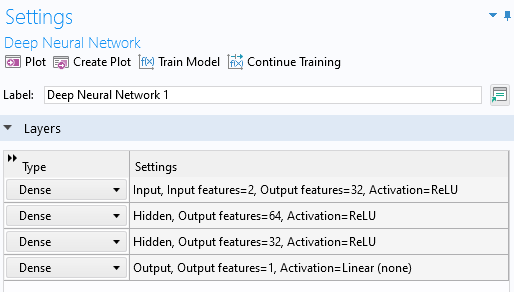
The network layer configuration using ReLU and Linear activation functions.
In this case, the Learning rate is lowered to 1e-4, and the Number of epochs is set to 10,000.
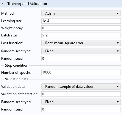
The Training and Validation section settings for the network using the ReLU and Linear activation functions.
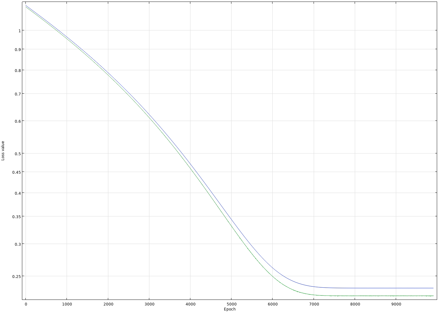
 A line graph containing one blue line and one green line with the epoch number on the x-axis and loss value on the y-axis.
Convergence plot for the network using the ReLU and Linear activation functions.
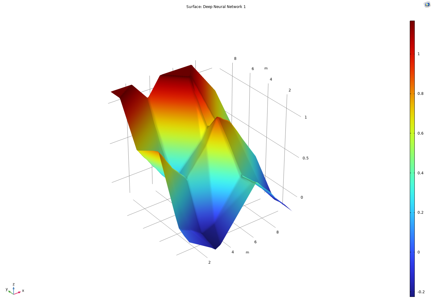
This network is easier to train but gives a larger loss than when using the tanh activation function. A certain level of overfitting is seen in this case. When using the ReLU and Linear activation functions, the resulting surface is piecewise linear with resolution determined by the size of the network, as shown in the figures below for a few different network configurations. The network configurations used are ,  , and
, and  . Reducing the model complexity further results in underfitting.
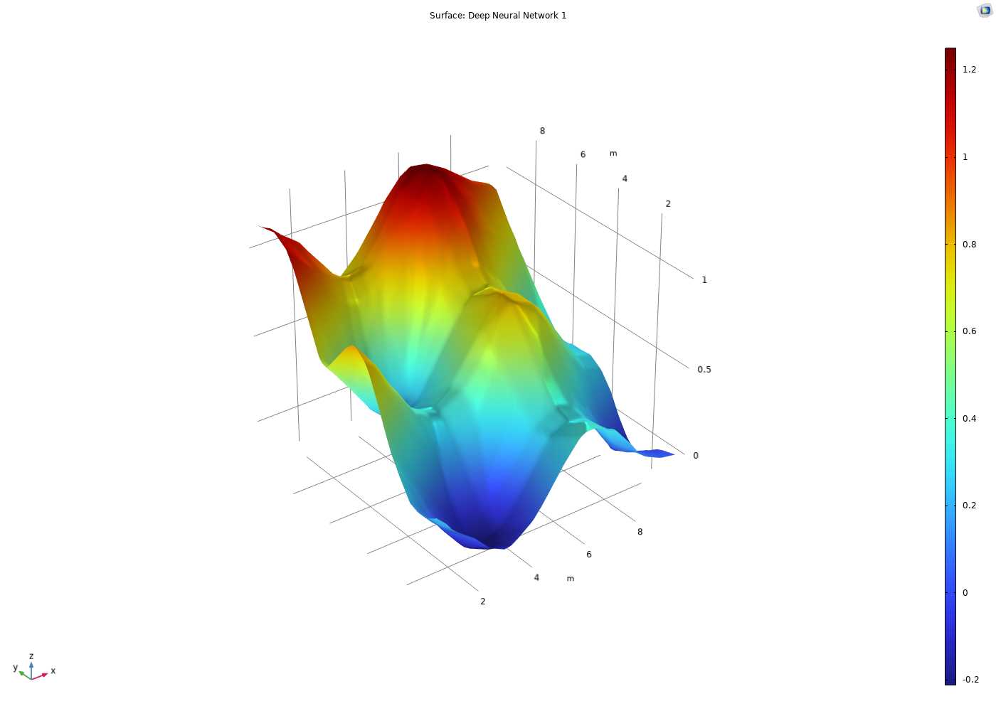 A rainbow-colored, smooth surface plot with a few hills and valleys.
The function surface when the ReLU and Linear activation functions are used for a network.
 A rainbow-colored, smooth surface plot with a few hills and valleys.
The function surface when the ReLU and Linear activation functions are used for a network.
 A rainbow-colored, smooth surface plot with a few hills and valleys.
The function surface when the ReLU and Linear activation functions are used for a network.
If we use a very simple  network, we get an underfitted model. The loss stalls at a relatively high level of about 0.2, as seen in the convergence plot below.
 This is not the greatest caption in the world. A line graph containing a blue line and green line with the epoch number on the x-axis and loss value on the y-axis.
The convergence of a network stalls at a loss value of 0.2.
The network complexity is too low to accurately represent the data. The resulting neural network function is a virtually constant function when using the same solver parameters. This is shown below.
 A rectangular surface plot in 3D space with a rainbow color distribution, of which the majority is a dark red color.
The underfitted network model results in a virtually constant function.
You can observe this firsthand in the model file for the ReLU and Linear activation functions, here.
请提交与此页面相关的反馈,或点击此处联系技术支持。