Using Symmetry to Improve Simulation Time
To reduce the computational time and resources required to compute a model, there are several strategies you can employ as well as features in the COMSOL Multiphysics® software that you can use. Here, we demonstrate how to take advantage of the symmetries in your optical scattering models to simplify computation.
Tutorial: Use Symmetry to Improve Simulation Time
Using the completed model built at the end of Part 4 of this course, follow along in the software as we show how to take advantage of symmetries in an optical scattering model. The memory and time required to compute the model are reduced through implementing symmetry boundaries. Important steps in building this model include preparing the geometry, defining the symmetry plane, and expanding the results plots to visualize the entire modeling domain. These steps will be discussed further after the tutorial.
Prepare Geometry
Before adding the appropriate boundary conditions that will enable you to reduce the modeling domain, you must prepare the geometry. Due to the symmetry of the nanoparticle and physics boundary conditions, instead of modeling the entire sphere you can reduce the model size by a quarter. To do this, a block is added as a tool object in the geometry — placed so that it overlaps with the desired quarter of the region of the sphere — and an Intersection operation is used.
 A quarter of a small, gray sphere enclosed by a quarter of a larger, gray sphere.
The geometry for the model of a gold nanoparticle, reduced to a quarter of the sphere.
Define Symmetry Planes
To add perfect electric conductor (PEC) and perfect magnetic conductor (PMC) boundaries as symmetry planes, we add two Symmetry Plane boundary conditions to the model and specify the type of symmetry in the settings.
 A transparent quarter sector of a sphere with the boundaries on the bottom of the sector selected.
 A quarter sector of a sphere with the vertical boundaries along the sector selected.
The geometry selection for the PEC (left) and PMC (right) conductor boundaries to exploit symmetries in the model.
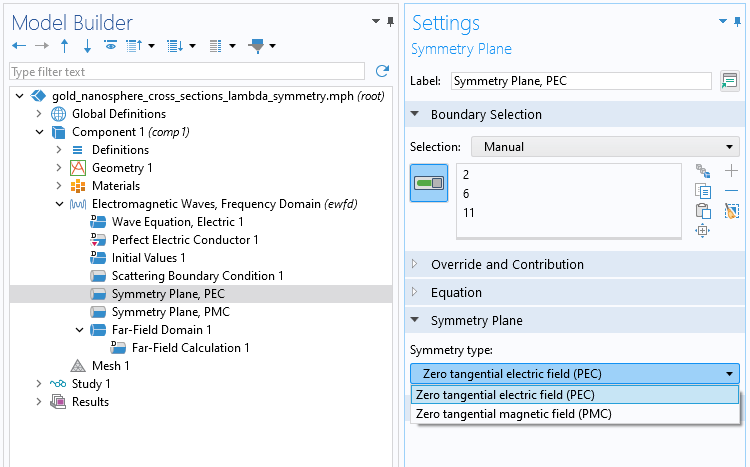
The options for the Symmetry type setting for the Symmetry Plane boundary condition.
The Perfect Electric Conductor boundary condition sets the tangential component of the electric field to zero. It imposes symmetry for magnetic fields. The Perfect Magnetic Conductor boundary condition sets the tangential component of the magnetic field to zero. It imposes symmetry for electric fields. Additional information on the PEC and PMC boundary conditions can be found in the resources outlined in the Further Learning section of this article.
Far-Field Analysis
For the far-field calculation, when the Symmetry Plane feature is used, these symmetries are automatically detected and taken into account upon changing the symmetry settings to From symmetry plane(s).
 A screenshot of the Model Builder with the Far-Field Calculation node selected, the corresponding Settings window, and both the boundary selection and radiation pattern displayed in the Graphics windows.
The settings for the Far-Field Calculation subnode. The symmetry settings are taken from the symmetry planes previously defined in the model.
Further Learning
- Learning Center:
- Documentation:
- Wave Optics Module > User's Guide > "Wave Optics Interfaces" > "The Electromagnetic Waves, Frequency Domain Interface"
- "Symmetry Plane" chapter
- "Perfect Electric Conductor" chapter
- "Perfect Magnetic Conductor" chapter
- Wave Optics Module > User's Guide > "Wave Optics Interfaces" > "The Electromagnetic Waves, Frequency Domain Interface"
- Tutorial models:
- Optical Scattering off a Gold Nanosphere (for PEC/PMC)
- Cloaking of a Cylindrical Scatterer with Graphene (for 2D axisymmetry)
请提交与此页面相关的反馈,或点击此处联系技术支持。