学习中心

Setting Up an Optical Scattering Model

---

Simulating optical scattering in COMSOL Multiphysics^® involves the standard modeling workflow: setting up, building, and then computing the model. See a step-by-step demonstration of this process and learn about using the scattered-field formulation here.

Tutorial: Optical Scattering off a Gold Nanosphere

Follow along in the software as we quickly build an example application featuring a typical gold nanosphere to present the basic workflow of optical scattering analysis in COMSOL Multiphysics. Important aspects of defining the computational model for this application include the scattered-field formulation, background field, and absorbing layer settings, which are all highlighted following the tutorial.

Choosing the Scattered-Field Formulation

For problems where a known background field is illuminating an object in free space, it is possible to use the scattered-field formulation. The known background field becomes a source term, and the scattered-field formulation thus solves for the relative electric field:

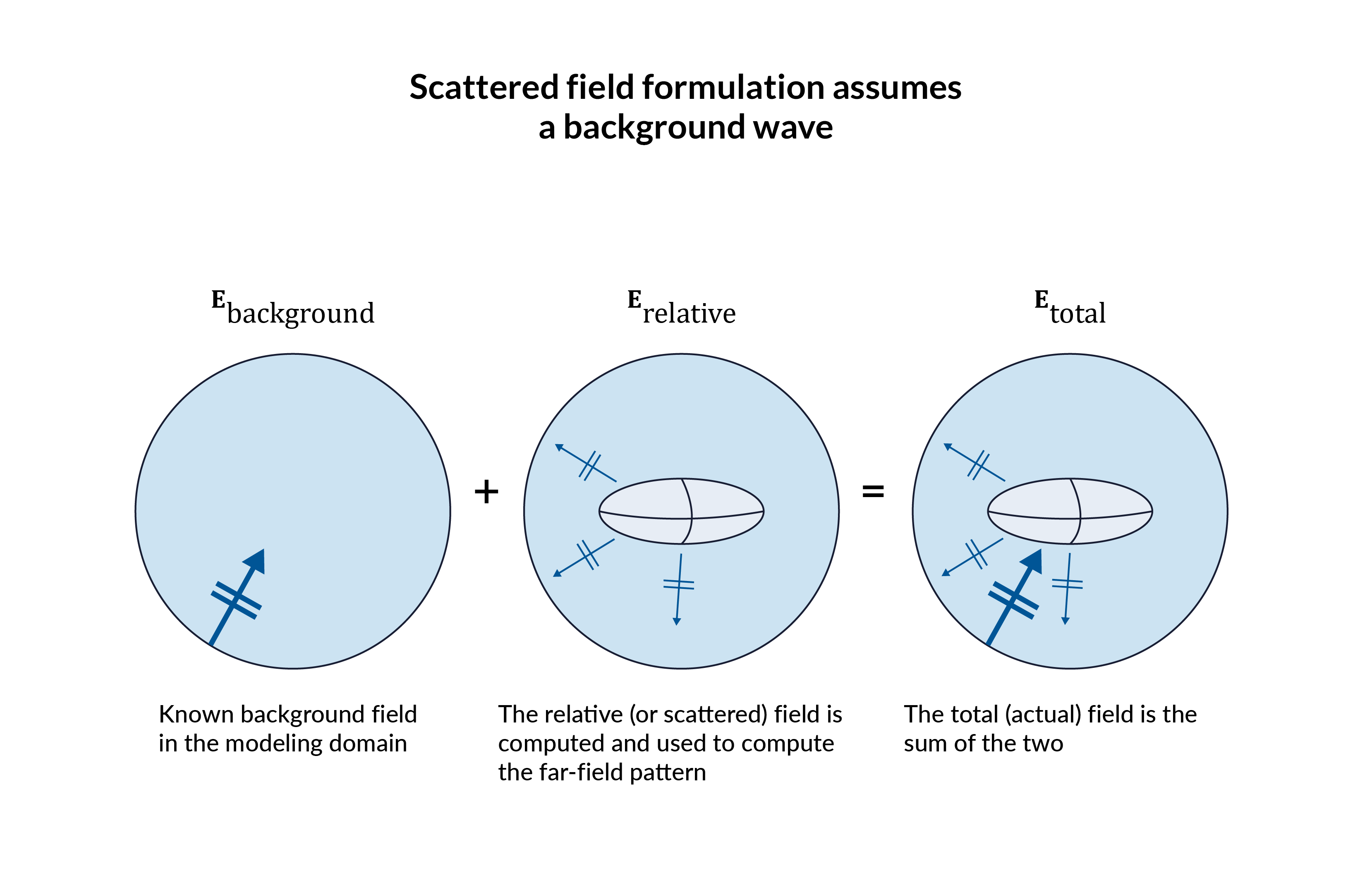Three light blue circles containing dark blue arrows and lines, with the second and third circles also containing a gray ellipsoid.

Visualization of the components of the total electric field.

The Settings window for the Electromagnetic Waves, Frequency Domain interface with the Formulation section expanded.

The Scattered field formulation is selected in the settings for the Electromagnetic Waves, Frequency Domain interface.

Defining the Background Field

There are different options available when specifying the background field. As seen in the image below, a linearly polarized plane wave background field, a paraxial-approximate Gaussian beam, or a user-defined background field can be selected. A linearly polarized plane wave is specified for this example.

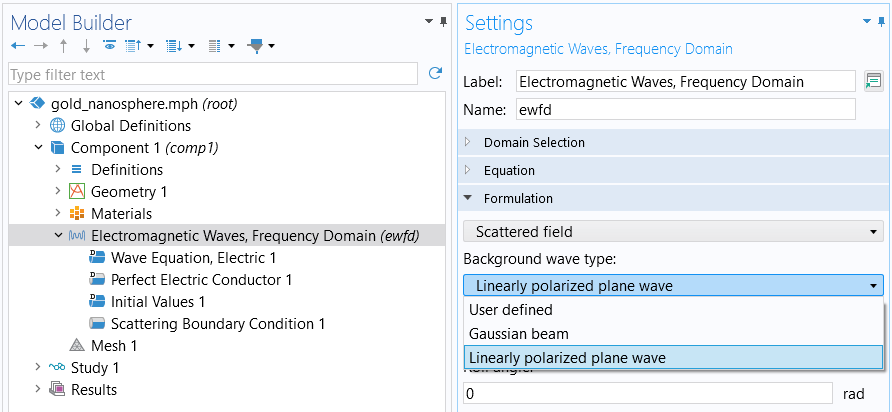
Options for the background wave type for a scattered field.

Defining the Absorbing Boundary Condition

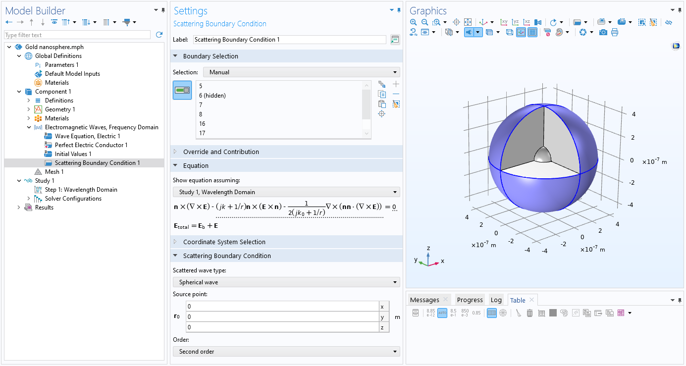
To collect the scattered light, an absorbing layer is defined at the outer boundary of our modeling domain. The absorbing boundary is typically placed at least half a wavelength away from the scatterer to avoid nearfields.

The Model Builder with the Scattering Boundary Condition node selected and the corresponding Settings window.

Settings for the Scattering Boundary Condition feature.

For this application example, we choose the Scattering Boundary Condition. We select the Spherical Wave type to fit our geometry. Choosing the second order improves absorbance slightly by taking into account an additional expansion term.

Tutorial: Adding a Perfectly Matched Layer

We now extend the model by adding a perfectly matched layer (PML). This enables you to further improve on avoiding reflections back into the simulation domain and pick up the scattered fields. Avoiding reflections leads to improved absorbance at higher angles of incidence but requires the definition of an additional geometric domain, as demonstrated in the tutorial below. The PML becomes necessary if you want to make sure that nonplane waves, such as evanescent fields, are absorbed appropriately. That also allows a much closer placement of the PML to the scatterer. Follow along to learn how you can simply add a PML to your existing model.

For further discussion on this topic, we highly recommend the blog post found under the resources for further learning.

Further Learning

• COMSOL Documentation:
  • Wave Optics Module > User's Guide > "Wave Optics Modeling" > "Scattered Field Formulation"
• Blog post:
  • "Using Perfectly Matched Layers and Scattering Boundary Conditions for Wave Electromagnetics Problems"
• Tutorial model:
  • Optical Scattering off a Gold Nanosphere