学习中心

Far-Field Analysis

---

Using COMSOL Multiphysics^® and the Wave Optics Module, a Far-Field Domain feature can be added to your model and used to plot the radiation pattern and 3D far field of your optical scattering models. In this article, you will see a demonstration of this, in which we expand on the base application built at the start of this course.

Tutorial: Calculating Far-Field Scattering

Follow along in the software using the completed model built in Part 1 of this course (the optical scattering off a gold nanosphere) as we demonstrate how to compute the far-field scattering. Important steps of building the model include defining the far-field domain, defining the far-field calculation, and plotting the far field. All of these steps are discussed further following the tutorial.

Defining the Far-Field Domain

In order to calculate far-field scattering, a Far-Field Domain node must be added to the model tree. After which we need to select the applicable geometry regions to specify the far-field domain. The homogeneous free-space domain between the scatterer and the absorbing layer is selected.

A screenshot of the Model Builder with the Far-Field Domain node highlighted and the geometry selection displayed in the Graphics window.

The Far-Field Domain node in the optical scattering model. The gold nanosphere in the center is removed from the geometry selection (domain number 5).

Defining the Far-Field Calculation

The far-field calculation is added by default under the Far-Field Domain node. It also requires a boundary selection for the outfacing boundary of the far-field domain. Note that symmetry planes can be taken care of automatically.

A screenshot of the Model Builder with the Far-Field Calculation node highlighted and the geometry selection in the Graphics window.

The Far-Field Calculation subnode settings.

By default, the outside boundary relative to the domain is used for the calculation and should be selected accordingly. Alternatively, you could use the inside boundary choice and select the surface of the scatterer instead.

Since the Far-Field Domain feature does not change the simulation itself, but simply introduces the new far-field variable Efar, you can choose update solution instead of compute to efficiently update the study results.

Plotting the Far Field

A plot of the electric field norm is generated by default upon computing an optical model. When the far-field domain is used in physics, additional radiation pattern plots are available by default if the study is run for the first time. The Reset default plots of the study node also creates them. They can be manually added as follows (also discussed in the video):

3D Radiation Pattern

To plot the scattering profile of our gold nanosphere, we add a 3D Plot Group node under the results. Then, we choose the Radiation Pattern plot type from the options available for volume plots.

A screenshot of the Model Builder showing the settings and results for the Radiation Pattern plot with annotations in the Settings window and Directivity results table.

The 3D radiation pattern for the far field. The results for the directivity and the expression used to calculate it are highlighted.

The directivity can automatically be calculated for the expression of interest. For optics, the default corresponds to the scattered power and uses the following expression: ewfd.normEfar^2.

2D Radiation Pattern

You can also plot the radiation pattern of the gold nanosphere in 2D. To do so, add a Polar Plot Group node under the results and add a Radiation Pattern plot again. The evaluation plane is defined by a normal vector and a reference direction.

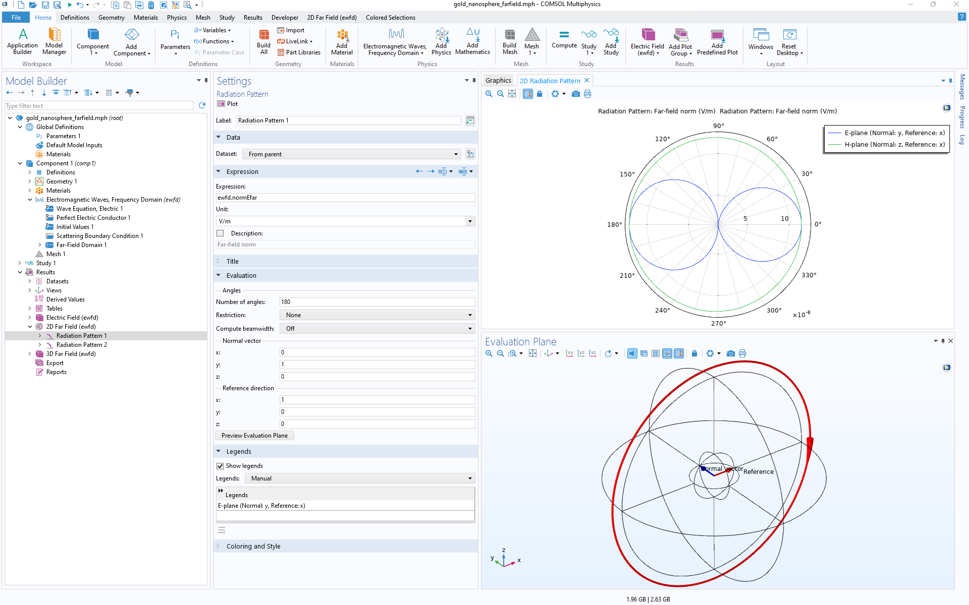A screenshot of the Model Builder with the 2D Far Field results plot for the Radiation Pattern displayed in the Graphics window.

The Radiation Pattern plot (upper right) and evaluation plane preview (lower right).

To ease the quantitative analysis, it is often preferable to investigate 2D cross sections of the 3D plot. This enables you to focus on specific planes. Here, multiple Radiation Pattern plots are used to visualize the scattering of the electromagnetic field in the E-plane and H-plane when the wavelength is 700 nm.

Further Learning

See the resources below for more information regarding far-field analysis — namely the documentation for a theoretical background:

• Documentation:
  • Wave Optics Module > User's Guide > "Wave Optics Modeling"
    • "Scattered Field Formulation" chapter
    • "Special Calculations" section in the "Far-Field Calculations Theory" chapter
  • Wave Optics Module > User's Guide > "Wave Optics Interfaces" > "The Electromagnetic Waves, Frequency Domain Interface" > "Far-Field Domain"
• Tutorial model:
  • Optical Scattering off a Gold Nanosphere