学习中心

Calculating the Small-Signal Parameters of a Speaker Driver from FEA

---

While small-signal (or Thiele–Small) and large-signal parameters used in a lumped representation of a speaker driver are often obtained via measurement, we can also extract their values from detailed finite element models. In this part of the course, we discuss the analyses that enable you to calculate small-signal parameters, using the 2D axisymmetric model of a dynamic driver from Part 2 as an example. The extraction of large-signal parameters is discussed in the next part.

Small-Signal Electrical Parameters

The electrical parameters can be obtained by running an electromagnetic analysis of the driver (at the rest position) that uses a Small-Signal Analysis, Frequency Domain study. The study has two steps. The Stationary step calculates the stationary magnetic field generated by the permanent magnet. In the Frequency Domain Perturbation study step, the voice coil (fixed or blocked) is excited with a harmonic AC voltage, and the perturbated magnetic field and the additional currents induced in the electromagnetic circuit are solved. The steps can be seen in the images below, and in the model file attached to this article, they are included under the Blocked Coil Magnetic Fields study.

Study steps for extracting small-signal electrical parameters.

Let's now derive the formula that can be used to calculate the force factor from this analysis.

Based on the Lorentz force law, a straight wire carrying an electric current, , in a uniform magnetic field, , experiences the Lorentz force

where is a vector whose magnitude is the length of the wire and whose direction is along the wire, aligned with the direction of the current in the wire . The term gives the so-called force factor, denoted as , which is the product of the magnetic field flux perpendicular to the coil and the total length of the coil. The higher the value , the larger the force that is generated by a given current flowing through the voice coil.

For a curved wire and nonuniform , the force can be calculated as

where is the current density and the integral is evaluated over the volume occupied by the coil.

For this 2D axisymmetric case, with a current directed in the azimuthal direction, the Lorentz force on the coil is given by

where is the azimuthal current density through the cross section of the coil, and is the radial component of the magnetic flux density. The force is pointing in the z direction and is denoted as

For a homogenized coil that consists of a single copper wire having N₀ turns,

where the integral is taken over the coil domain's cross-section area in the rz-plane. Assuming is constant in the coil cross section of area A, it becomes

When we rewrite the driving force in terms of the coil current rather than the cross-sectional current density , we get

The force factor, , is therefore calculated as

This can be done by evaluating the surface average of the term over the coil domains, as shown in the image below. The dataset used for this evaluation, Study 1: Blocked Coil Magnetic Fields Study/Solution Store 1, is the solution of the Stationary study step. The evaluation returns a value of 10.485 Wb/m.

A Surface Average evaluation is used to calculate the force factor BL.

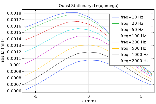
In the Frequency Domain Perturbation study step, coil parameters including the blocked coil impedance (mf.ZCoil_1), coil resistance (mf.RCoil_1), and coil inductance (mf.LCoil_1) are internally calculated and readily available for extraction in result analysis. The images below show plots of coil resistance (top), inductance (middle), and impedance (bottom) as a function of frequency.

Plots of coil resistance (top), coil inductance (middle), and coil impedance (bottom) as a function of frequency.

These frequency-dependent data can be used to define a lumped model, possibly in the following ways:

1. The data is used to calculate the lumped electromagnetic force that drives the transducer. One example is the Loudspeaker Driver in a Vented Enclosure tutorial we discussed in Part 5, in the section "Method Two: Using the Lumped Electromagnetic Force". We mentioned that two .txt files are imported into that model using two interpolation functions to define the frequency-dependent blocked coil resistance and inductance. These .txt files can be generated and saved from the plots of the blocked coil resistance and blocked coil inductance obtained here. You can either right-click the Export node in the Results tree and select Plot to export a selected plot's data, or right-click a desired plot and then select Add Plot Data to Export.

2. The data is used to estimate the required parameters that are used in a specific circuit model that represents the driver. For example, a simple LR model uses a constant resistance, , and a constant inductance, , to describe the electric impedance of the coil. The best estimate for the constant coil resistance and inductance for such a model can be obtained from the frequency-dependent impedance data obtained here . The coil resistance of the lowest study frequency (10 Hz in this case), 5.565 Ω , can be used as a good estimate for the DC resistance of the voice coil, as seen below.

Coil resistance extraction for low-frequency limit.

To get an estimated value for the inductance , we can use parameter fitting so that the frequency-dependent coil reactance calculated with the expression fits closely to the coil reactance (i.e., the imaginary part of the full coil impedance) obtained from the model . It can be done by adding a Least-Squares Fit node under Global Definitions with the settings shown below. This requires saving the coil reactance (imag(mf.ZCoil_1), or simply mf.XCoil_1) to a table beforehand and then pointing the data source to the table in the Least-Squares Fit settings. Here, the table is created through evaluating the coil reactance variable, mf.XCoil_1, using a Global Evaluation feature under Derived Values. Finally, click the Fit Parameters button in the Least-Squares Fit menu bar and the evaluation returns a value of 1.08e-3 H for .

Coil inductance is estimated by using the Least-Squares Fit feature (top) that fits the function to the coil reactance table created with a Global Evaluation node (bottom).

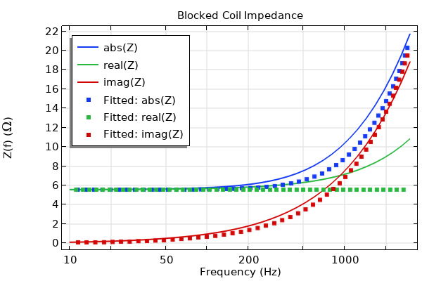
The image below compares the impedance calculated using the expression with the estimated and to that obtained directly from the model, indicating that 1.08e-3 H provides a good fitting for . Note that this is for the simple LR model for the coil. The circuit that is fitted to the data can also, for example, be a common so-called LR-2 or LR-3 model. You can of course always use the full frequency-dependent data , which will not require any model fits.

Coil impedance estimated using the fitted coil inductance compared to that calculated directly from the model.

Small-Signal Mechanical Parameters

An eigenfrequency analysis of the mechanical system enables you to obtain the fundamental resonant frequency, , and the mechanical Q-factor at , . Those quantities can then be used to calculate the resistance, , that simulates the mechanical damping in the lumped circuit model. To best capture the resonance and damping, the analysis should include the mechanical losses in the vibrating solids as well as the thermoviscous losses in the magnetic air gaps or other narrow regions present in the transducer when these are not specifically simulated in the FEM acoustic model. Note that any losses that are eventually captured in the FEM part of the model should not be included in the lumped speaker representation.

Whenever a system has energy loss, an eigenfrequency study returns eigenfrequencies as complex numbers with the imaginary parts representing the damping. In this example, we want to include the loss due to mechanical damping in the spider, surround, cone, and former as well as the thermoviscous loss in the narrow air gaps. Note that the thermoviscous loss is frequency dependent, which makes the problem depend nonlinearly on the eigenvalue (the frequency). To solve such a nonlinear eigenvalue problem, an iterative procedure is necessary in order to obtain accurate damped resonant frequencies. Basically, the nonlinear problem needs to be linearized around a value, called a linearization point in COMSOL Multiphysics^®. You start with something close to the resonance and use it as the linearization point to solve the full nonlinear eigenvalue problem. For highly nonlinear cases, you may need to run the solver repeatedly, updating the eigenvalue linearization point to the last eigenvalue found, until the eigenvalue converges.

It is recommended to always start with computing the fundamental resonant frequency of the transducer without including the acoustic load and damping (as it is operated in vacuum). This gives you the loss from mechanical damping of the solid parts only and allows you to calculate when the thermoviscous acoustic damping should not be included. It also provides a good starting linearization point for the nonlinear study when the acoustic damping needs to be incorporated. Let's now look into how to run an iterative procedure and set up Eigenfrequency studies to find the damped fundamental resonant frequency.

Step 1

The first step is to run an eigenfrequency study just on the Solid Mechanics interface to search for the fundamental resonance frequency of the transducer when mechanical damping in solids is solely included. This is done by selecting only the Solid Mechanics interface in the Physics and Variables Selection edit area, as demoed in Study 2. In Study Settings, simply use the default settings for Eigenfrequency solver (ARPACK), Eigenfrequency search method (Manual in versions through 6.1, or Around shift in versions 6.2 and up), and Search for eigenfrequencies around (1 Hz) . Enter 1 in the Desired number of eigenfrequencies edit area, and select Larger real part for Eigenfrequency search method around shift. This way, the solver will find the lowest eigenfrequency of the transducer when it is operated in vacuum. In this case, the search returns one eigenmode at 53.237+12.696*i Hz.

Eigenfrequency study settings to compute the fundamental resonant frequency of the transducer operated in vacuum (top) and the search returns one resonant mode (bottom).

Step 2

The resonant frequency found in Step 1 is then used as the linearization point to solve the full nonlinear eigenvalue problem, as demoed in Study 3. In the Physics and Variables Selection edit area, now also select the Pressure Acoustics, Frequency Domain interface as well as the Acoustic-Structure Boundary multiphysics coupling in addition to the Solid Mechanics interface, as seen in the top image below. In the Study Settings section of the Settings window, enter the found resonant frequency in Step 1, 53.237+12.696*i , in the Search for eigenfrequencies around field; enter 2 for Desired number of eigenfrequencies; and select Closest in absolute value for Eigenfrequency search method around shift. Then, in the Eigenvalue solver node, set Value of eigenvalue linearization point to 53.237+12.696*i (the middle image). Compute the study and the searchreturns with a new value for the same mode at 53.237+12.696*i Hz (the bottom image). Note that the settings used here are sufficient for finding the desired mode. When necessary, increase the number for the Desired number of eigenfrequencies setting to ensure that the wanted mode is found. In this case, the eigenvalue solver also finds other modes that have different mode shapes than the one we looked for, so those can be discarded.

Eigenfrequency study (top) and Eigenvalue Solver (middle) settings to solve the nonlinear eigenvalue problem when the thermoviscous damping is included. The search returns a new resonant frequency (bottom).

Step 3

Enter 50.059+11.289*i in:

• The Search for eigenfrequencies around field in the settings for the Eigenfrequency study
• The Value of eigenvalue linearization point field in the settings for Eigenvalue Solver

Then, run the study again. The new search yields the same result, indicating we've reached a converged solution.

Solving a nonlinear eigenvalue problem requires updating the eigenvalue linearization point to the last eigenvalue found until the eigenvalue converges.

We now have the fundamental resonant frequency to be , and from this we can obtain

and

Note that the Q-factor is also calculated internally and saved in the variable named solid.Q_eig.

Next, we discuss how to run a structural analysis in order to extract the mechanical compliance, . The compliance can be calculated as the ratio of change in coil displacement, , to change in total applied force, :

For this purpose, we apply a static body load to the coil (upper image below) and compute its deformation using a Stationary study (middle image). A Parametric Sweep is added to change the value of the applied force (bottom image) in order to obtain the change in coil displacement. In this linear analysis for small deformations, two values are sufficient.

A structural analysis is used to extract the mechanical compliance.

The difference in coil displacements for the two applied forces are then used to calculate the compliance, as seen below. The with operator is used in the expression to access the solution of the first (having 1 as the first argument) and the second (having 2 as the first argument) force values. Here, we choose to use the solution at a point in the coil domain for this evaluation. Using any point in the moving structure should give a very similar answer since the whole structure moves together for low frequencies when a lumped model is valid.

The evaluation of coil compliance.

An integration of the density over all moving structure domains gives the total mechanical mass, , as seen below. Make sure the Compute volume integral box (in the Integration Settings section of the Surface Integration Settings window) is checked to compute the integral that takes the axial symmetry into account.

The total mechanical mass is obtained by integrating density over all moving structure domains.

Finally, we are able to calculate the mechanical resistance, , using the following relations:

and

With known , , and , can be calculated as

where .

The parameters extracted directly from the model are stored in the Parameters: TS Parameters (extracted from model) node in the attached model file, which are also shown in the image below.

Thiele–Small parameters extracted directly from the finite element analysis.

The image below shows the other parameters that are derived from the extracted parameters. They are stored in the Parameters: TS Parameters (derived) node in the attached model.

Thiele–Small parameters derived from the extracted parameters.

The effective radius of the driver is measured directly from the geometry. It is the radius of the diaphragm aperture plus half of the surround.