Fundamentals of Swept Meshing
The COMSOL Multiphysics® software contains many features and functionality that enable you to generate different types of meshes. Depending on the application, certain mesh types will be better suited and provide advantages for discretizing your model geometry, such as requiring significantly less memory when solving the model. One of these mesh types is a swept mesh. So, what exactly is a swept mesh and when should you consider using one in your model? In this article, we will address questions such as these and more.
What is Swept Meshing?
For now, let us consider a simplified definition of swept meshing in order to get a quick grasp of this operation. Swept meshing is a process that can only be applied when working with 3D geometries, and it involves extruding a surface mesh throughout the domain. It is only possible to build a swept mesh if the geometry domains meet certain criteria. This is addressed in Part 2 of this course on swept meshing, along with a third part focusing on rules and procedures for how to build swept meshes.
This 3D geometry of a single conductor coil is swept meshed by sweeping the cross section. Since the surface mesh was meshed with triangles, the resulting volume mesh is composed of prisms.
By construction, a swept mesh is a type of structured or semistructured mesh composed of prisms or hexahedrons. By structured, we mean a mesh where the interior mesh vertices are adjacent to the same number of elements. The mesh is structured in the sweep direction and then either structured or unstructured orthogonally to the sweep direction.
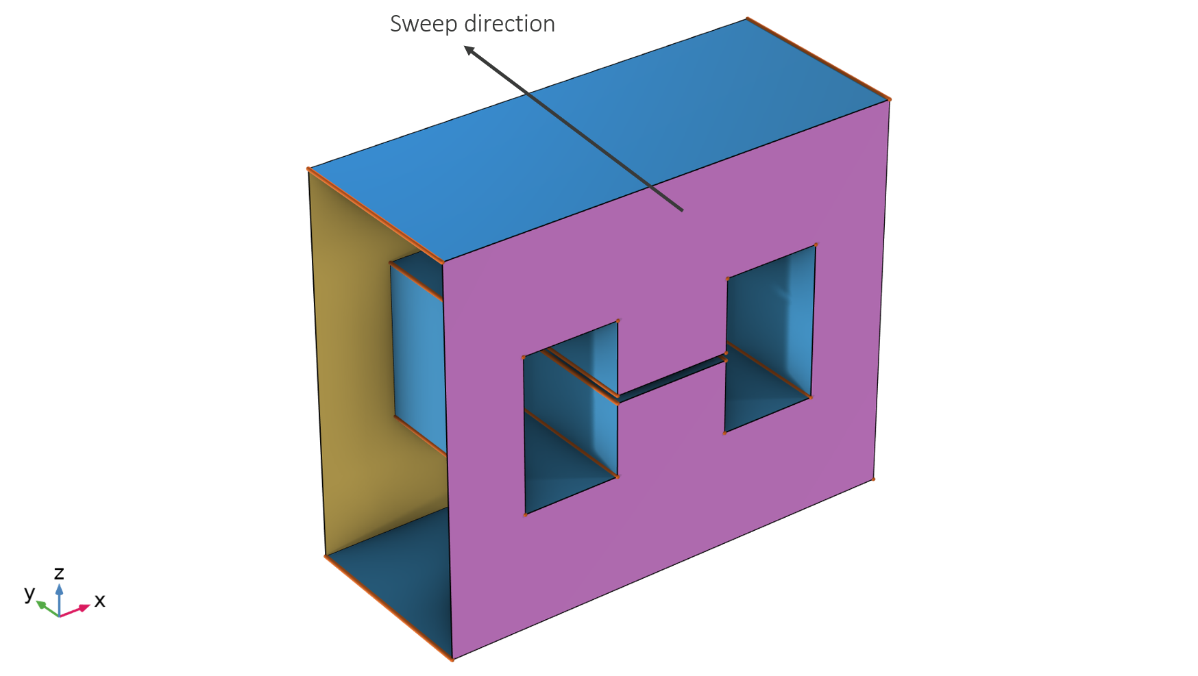
An outline of the process of swept meshing: A magnetic core with an air gap.
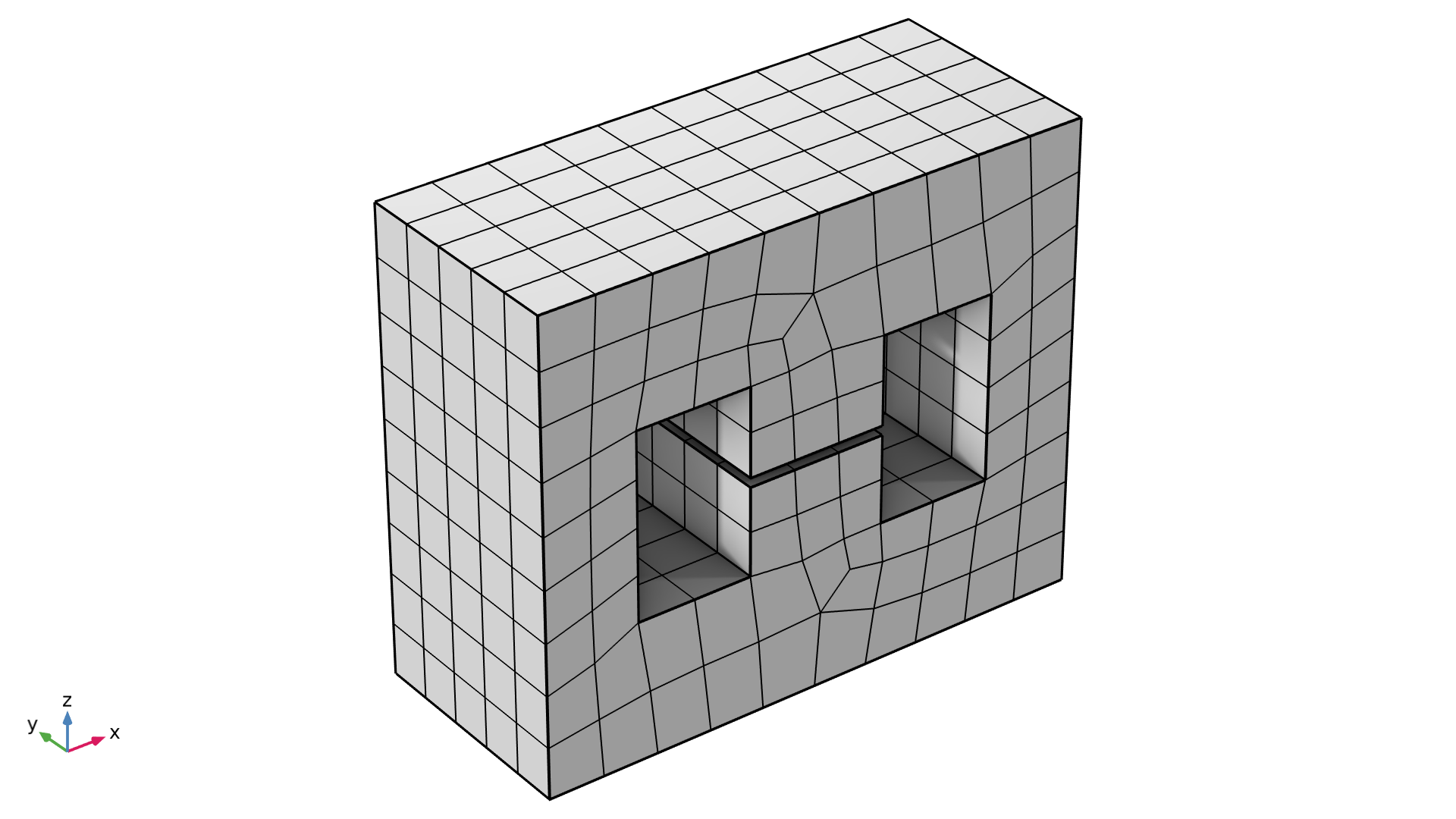 A 3D magnetic core geometry with a cross section that has an unstructured mesh made of quad mesh elements.
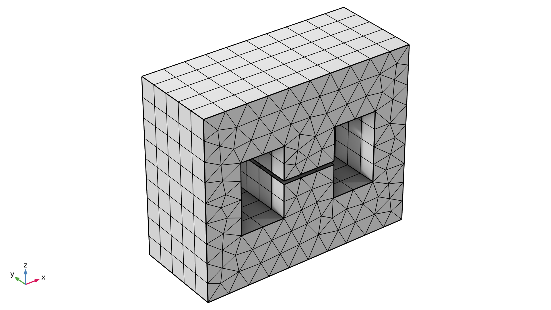 A 3D magnetic core geometry with a cross section that has an unstructured mesh made of triangle mesh elements.
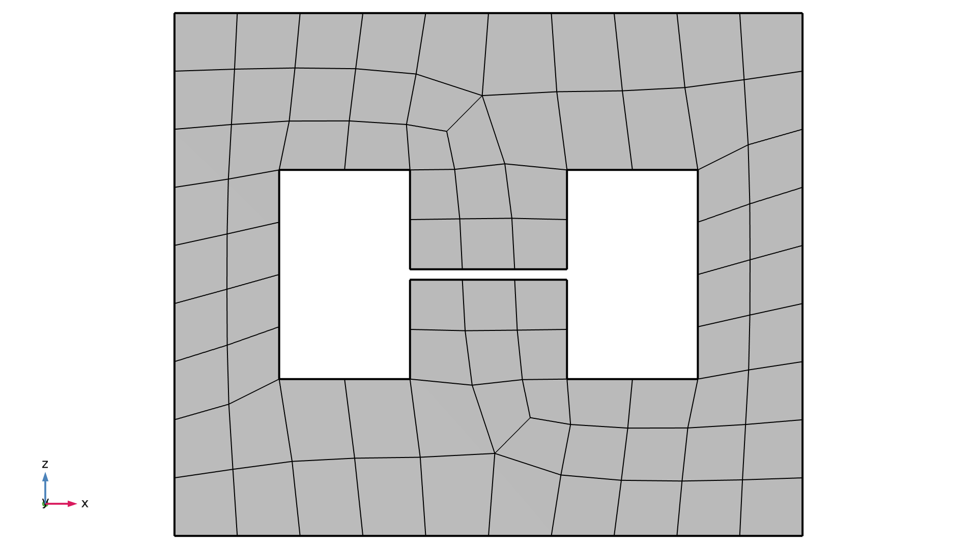 A close-up of the cross section for the unstructured mesh made of quad mesh elements.
 A close-up of the cross section for the unstructured mesh made of triangle mesh elements.
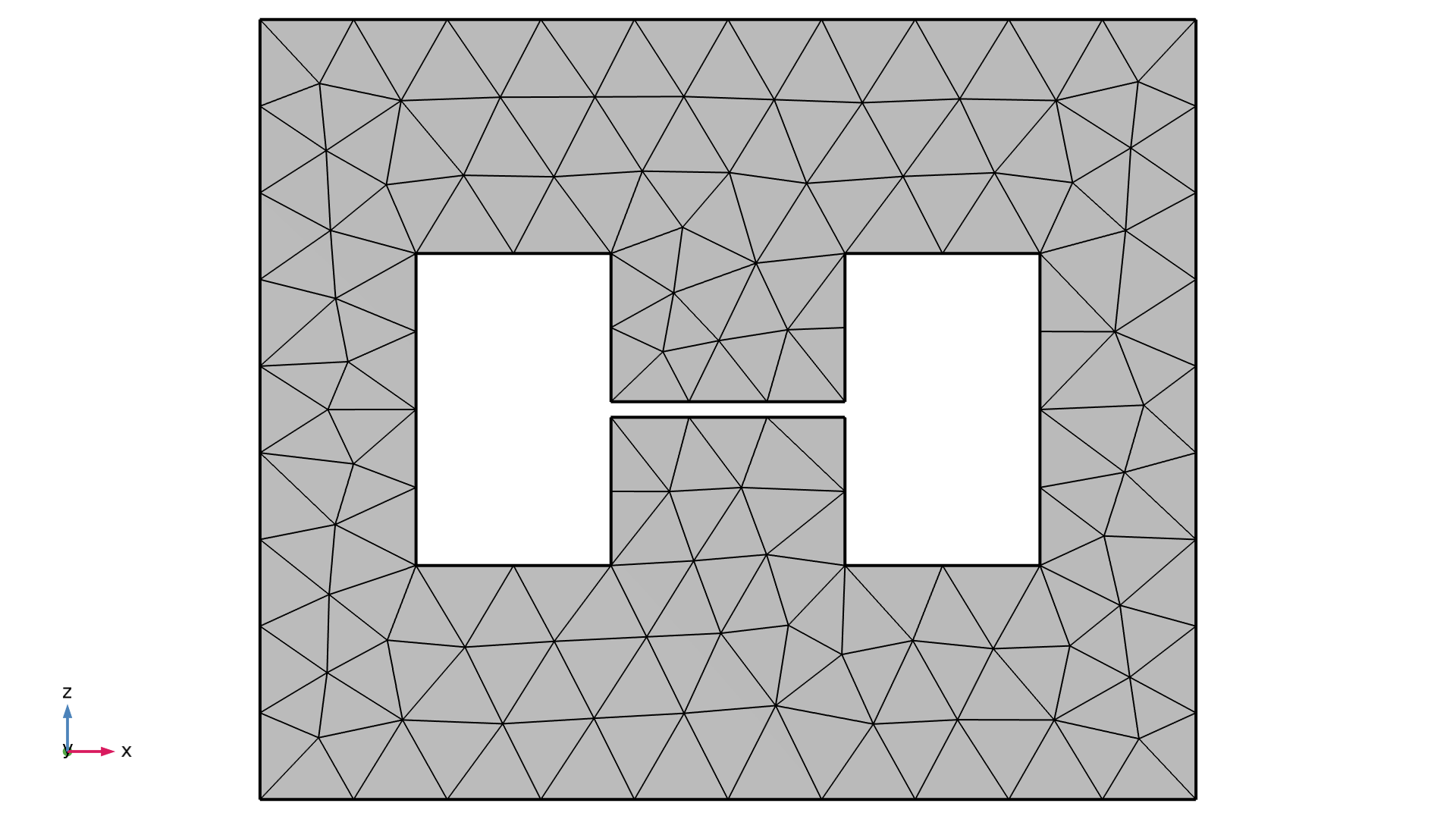
A magnetic core is swept meshed along the y direction. In most cases, the mesh on the cross section is unstructured for any mesh element type being used, as shown here. In the upper-left figure, the cross section has an unstructured mesh made of quad mesh elements, whereas it is made of triangle mesh elements in the upper-right figure. In both cases, the mesh along the sweep direction is structured. The lower figures show a view of the cross section for the two types of unstructured meshes.
 A 3D magnetic core geometry with a cross section that has an structured mesh.
 A close-up of the cross section for the Structured mesh.
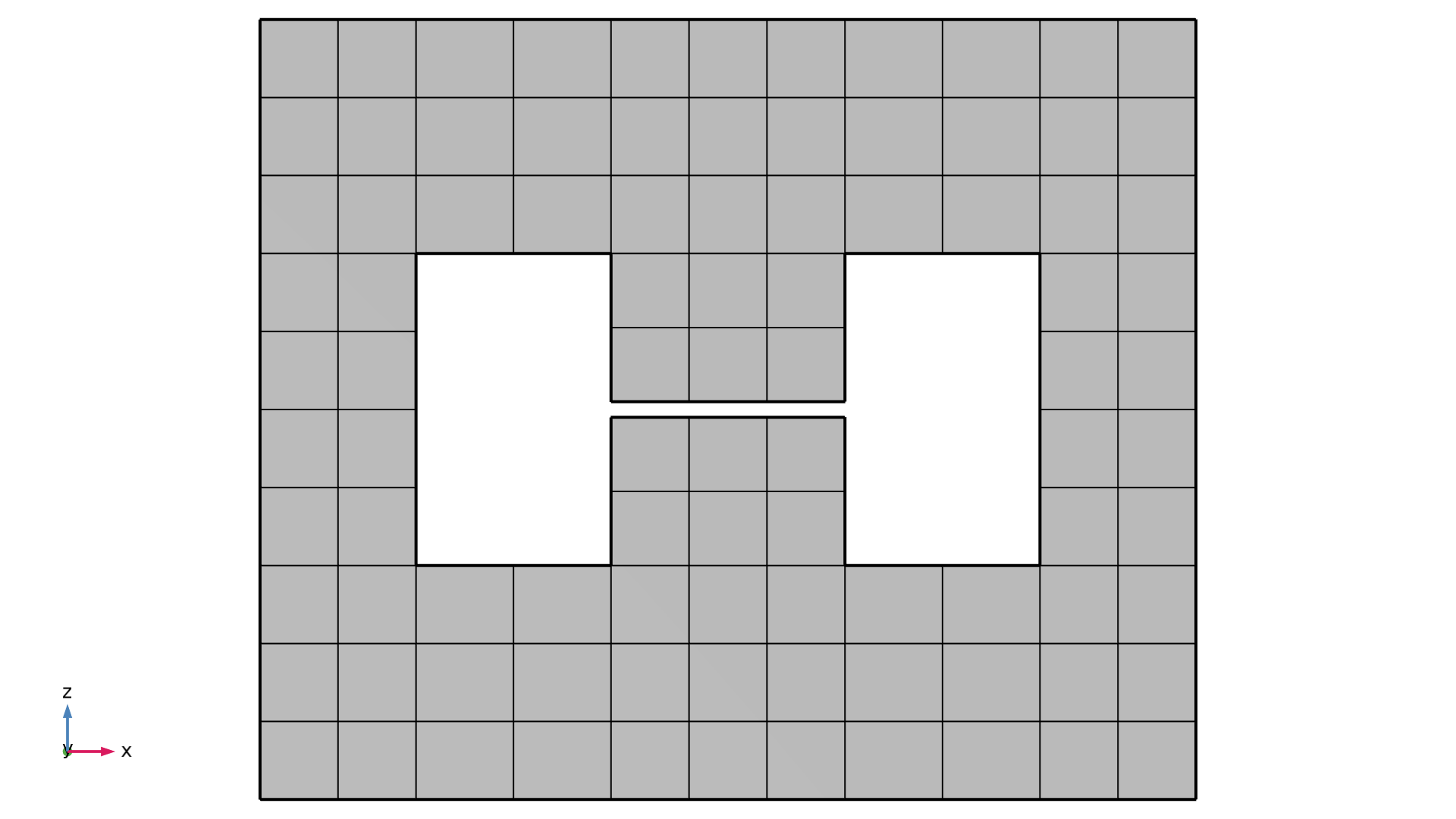
The same geometry can also be swept meshed using a structured mesh. While it is also composed of quad mesh elements like one of the previous unstructured meshes, this mesh is structured on the cross section as every interior mesh vertices are adjacent to 4 mesh elements. Such a structured mesh is either generated automatically if the face has an adequate topology or by first adding a Mapped operation on the source face, before the Swept operation.
Now that we have reviewed the concept of what a swept mesh is, let us explore examples of and use cases for swept meshing.
Advantages and Examples of Swept Meshes
The purpose of the swept mesh is to represent the geometry and solution of the computed fields with accuracy, while using minimal computational resources. In some cases, the default tetrahedral mesh generated is either not good enough to capture the gradients in the solution, for example, or is too computationally expensive to allow the model to be solved on standard machines in an acceptable amount of time. When gradients are localized, both of these can be true. Swept meshes offer a solution for this, and are applicable and relevant for any physics application area.
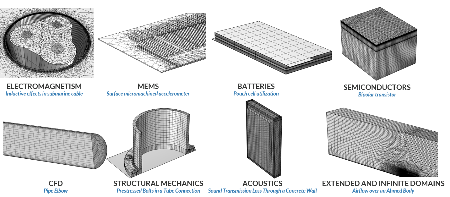 Eight tutorial models that use swept mesh; the examples shown include electromagnetism, MEMS, batteries, semiconductors, CFD, structural mechanics, acoustics, and extended and infinite domains.
Tutorial models examples (for different application areas) that use a swept mesh. You can find each of these tutorial models in the application libraries.
While swept meshes might give the impression that they are the universal solution to all or most models, there are still some cases where a tetrahedral mesh is recommended instead. For instance, a tetrahedral mesh would be better in cases that involve:
- Complex topology
- A mesh that needs to grow in size at different rates depending on the location and direction
Note that these cases may only occur in some portion of the geometry, while the rest can be swept meshed. In that case, different mesh types can be combined in order to implement the best elements of each.
For a swept mesh, there are three major advantages, regardless of the physics you are solving. For instance:
- Using it results in a low number of mesh elements.
- Using it results in good-quality elements in thin geometries.
- It is efficient to generate.
Let us go through each advantage in more detail.
Low Number of Mesh Elements
For any type of volume mesh that is homogenous in size (i.e., all elements have the same size), the number of elements,  , is proportional to the total volume to be meshed,
  , and inversely proportional to the cube of the typical mesh size,
  :
:

This constant of proportionality is of interest to us. It can be shown that for a given mesh size and volume:
- A prism mesh will consist of 1/7 of the amount of elements as a tetrahedral mesh.
- A hexahedron mesh will consist of 1/17 of the amount of elements as a tetrahedral mesh.
In reality, the mesh is almost never homogenous because of refinements due to the geometric complexities, but this gives a good order of magnitude.
The number of elements used to discretize a model domain affects the computational time and resources required to solve the model equations. However, this number alone is not really what matters when performing a study; the number of degrees of freedom (DOFs) is the governing number. For example, solving for the temperature field (using the energy conservation equation) means solving for a single DOF per computational point, whereas solving for solid mechanics means solving for at least three variables per computational point, which requires increased computational time and resources (when we use comparable solving strategies). Additionally, if the problem is nonlinear, we may find ourselves solving for a problem iteratively, resulting in an even more time- and resource-consuming simulation.
The placement of the element nodes for the three most common discretization types (linear, second-order Lagrange, and second-order serendipity) is depicted in the animation below:
Placement of the second-order Lagrange element nodes for different volume mesh elements (red, black, and blue points). If we remove the blue nodes, we obtain the corresponding serendipity elements. The linear element nodes are depicted with red points; they correspond to the mesh vertices.
Notice that for any of the three discretization types, prism and hexahedron elements contain more DOFs per element, but this is compensated by the fact that there are less elements in total in a swept mesh. Overall, the net gain is lower than the one we could have hoped for after comparing the number of mesh elements, but this is still significant. Notice also that a tetrahedral element with serendipity discretization has the same number of DOFs as a tetrahedral element with Lagrange discretization. This means that the net gain of swept meshes with serendipity discretization is even more significant.
It can be shown that a homogenous mesh composed of prisms or hexahedra, compared to a homogenous mesh composed of tetrahedra with same discretization and size, requires:
- Around 1/2 the number of DOFs, using linear or quadratic Lagrange discretization
- Around 1/4 the number of DOFs, using quadratic serendipity discretization
Good Quality Elements in Thin Geometries
When is the Quality "Good"?
Throughout this section and course, we should keep in mind that the quality metrics are more of a hint of what matters for a simulation than something that is absolutely known. The interpretation of this measure will depend on the model and the type of physics being solved. Because of this, when we write that a mesh is "good", this means that the user followed the field guidelines and the current state-of-the-art in mesh quality.
Good element quality is something we should strive to achieve, as this quantity influences the robustness of the numerical problem. As a rule of thumb, the mesh should result in a well-conditioned stiffness matrix. (The mesh quality is a good indication of this.) A broader discussion on what constitutes a quality mesh is outside the scope of this course, but is one of the fundamental topics of numerical analysis.
The mesh should have the lowest number of elements, yet use a sufficient amount to still be accurate enough to provide reliable solutions. The mesh elements should also be of good quality, as higher quality meshes provide better convergence. Note that these properties are in general conflicting and require you to use your own engineering judgement to decide on what is the best compromise between them.
Prisms or hexahedra, which compose a swept mesh, can be of good skewness quality even when the element is very flat. In other words, they can be stretched or compressed along one direction, and their skewness quality will not be impaired, unlike with tetrahedra.
From left to right: a tetrahedron, prism, and hexahedron mesh element are being vertically compressed from an optimal shape (all length equal) to a flat version.
Other types of quality measures (such as volume versus length) report a low mesh quality — even for swept elements — because those measures take the aspect ratio (ratio between the longest and smallest length) into account. With this, it seems that we arrive to a contradiction. So, what is the quality measure to "trust"? It depends.
In a general case, the ratio between largest and smallest coefficients of the stiffness matrix are proportional to the square of the aspect ratio. In other words, the matrix can become ill-conditioned for elongated elements. From a physics point of view, swept meshes with a high aspect ratio should not be used in case the solution field has a strong cross gradient (a gradient diagonal to the element, which is not uncommon in most solid mechanics problems) because the solution might not converge or be accurate.
However, for other particular fields being solved, it might happen that the cross gradient is negligible. In that case, the skewness quality is a good indicator to follow (remembering that the prism and hexahedron elements keep a high value). Consequently, this means that a swept mesh enables us to use fewer elements, and less DOFs, while keeping the solution robust.
Quantification of the Benefits of Swept Mesh Elements on Thin Geometries
Let us suppose that the physics can use a mesh with elongated mesh elements. There are two cases of scenarios to consider.
This first scenario is for elongated geometries, such as cables and pipes. You would need to create a swept mesh with elements that are more or less stretched along the length of the geometry. Say, for example, that the aspect ratio of the swept mesh element is  , and the number of DOFs is
  less compared to tetrahedra. (
 for serendipity discretization.)
 Two stacked elbow pipe geometries with different meshes.
Comparison between two types of meshes for an elbow pipe geometry. The swept mesh (at the top) is composed of prisms with a length twice as long as their base (hence why  ). Compared to prisms with an aspect ratio of 1, this mesh has consequently around 2 times less DOFs if it is discretized with quadratic Lagrange elements. Overall, the swept mesh has 4 times less DOFs compared to the tetrahedral mesh (at the bottom).
The second scenario is for narrow geometries (plate-like geometries with a small thickness). For such geometries, the effect is even more noticeable. To be isotropic, the tetrahedra need to have at least the size of this small thickness, while swept elements can be large on the perpendicular directions of the sweep. For an aspect ratio, , of the swept mesh elements, the number of DOFs are now  lower! (
 lower for serendipity discretization.) This principle is also used when resolving high fluid velocity gradients near walls using a boundary layer mesh.
 Close-up of the corner of a geometry, showing swept mesh.
 Close-up of the corner of a geometry, showing unstructured tetrahedral mesh.
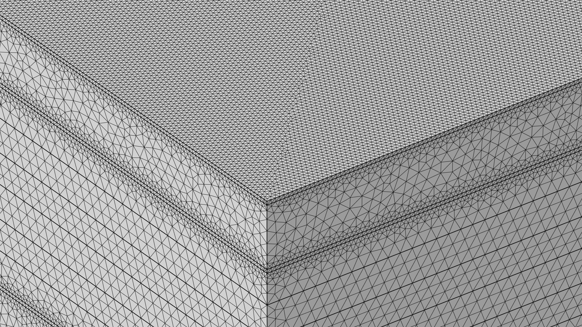
Comparison between two type of meshes for a resonator geometry, with each geometry zoomed in on a corner. The left image shows this geometry with a swept mesh using prism elements, whereas the right shows the geometry with an unstructured free tetrahedral mesh. In both cases, the meshes are resolving the depth with the same number of elements. However, the prisms have an aspect ratio of 50. This means that there are 2500 times less elements on the surface. Overall, this means that the mesh on the right would use around 5000 times more DOFs.
Efficient to Generate
In comparison with the tetrahedral mesher, where the insertion of interior nodes might take a long time for large meshes due to the fact that it is unstructured, a swept mesh is relatively quick to generate because it essentially only needs to mesh the boundaries, as the interior nodes are deduced automatically. This is a simplified explanation to fit the scope of this article. However, even though the mesh generation is faster, it might also necessitate further geometric operations in order for the geometry to be "sweepable". This part usually requires additional time that cannot be neglected in some cases.
Example
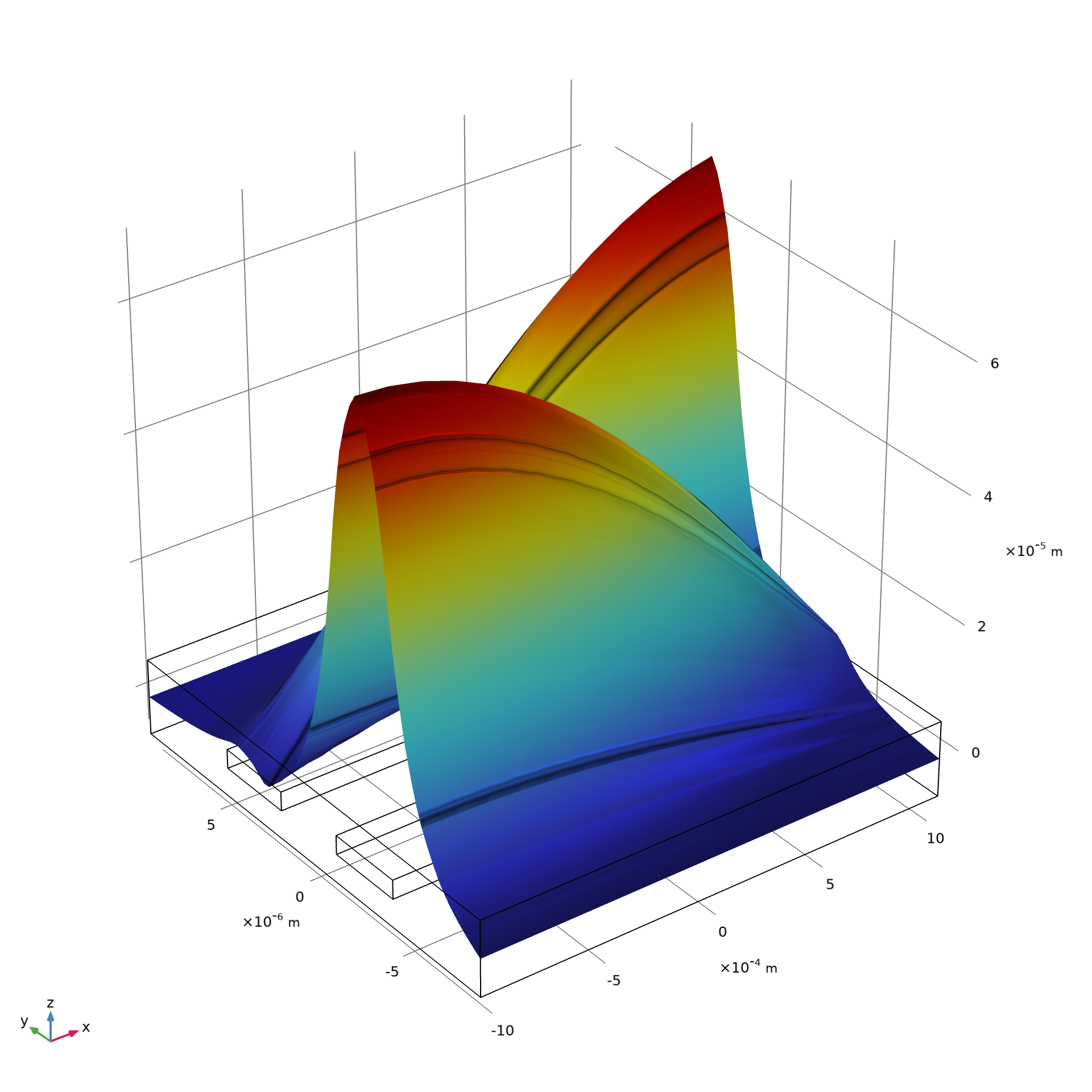
If used appropriately, swept meshing allows the meshing of different designs to be completed faster and require less resources in terms of RAM than other types of meshes, making our solution and overall product development process faster and leaner. The main takeaway is that, with this type of mesh, we can decouple the mesh discretization perpendicular to the sweep direction with the discretization along the sweep direction, which can be useful in many situations, as demonstrated below with the Surface Micromachined Accelerometer tutorial model. MEMS is a typical application where swept meshes are useful since they exhibit high aspect ratios.
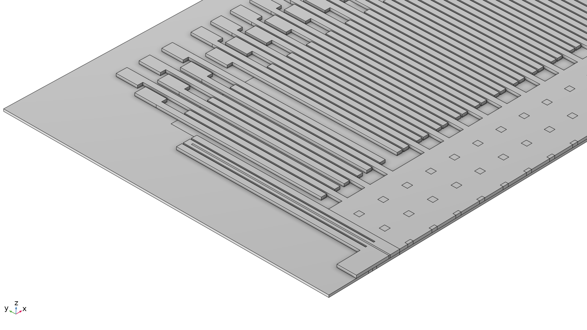 The geometry for the Surface Micromachined Accelerometer.
The model geometry for the Surface Micromachined Accelerometer tutorial model. The top air domains are hidden for visual purposes.
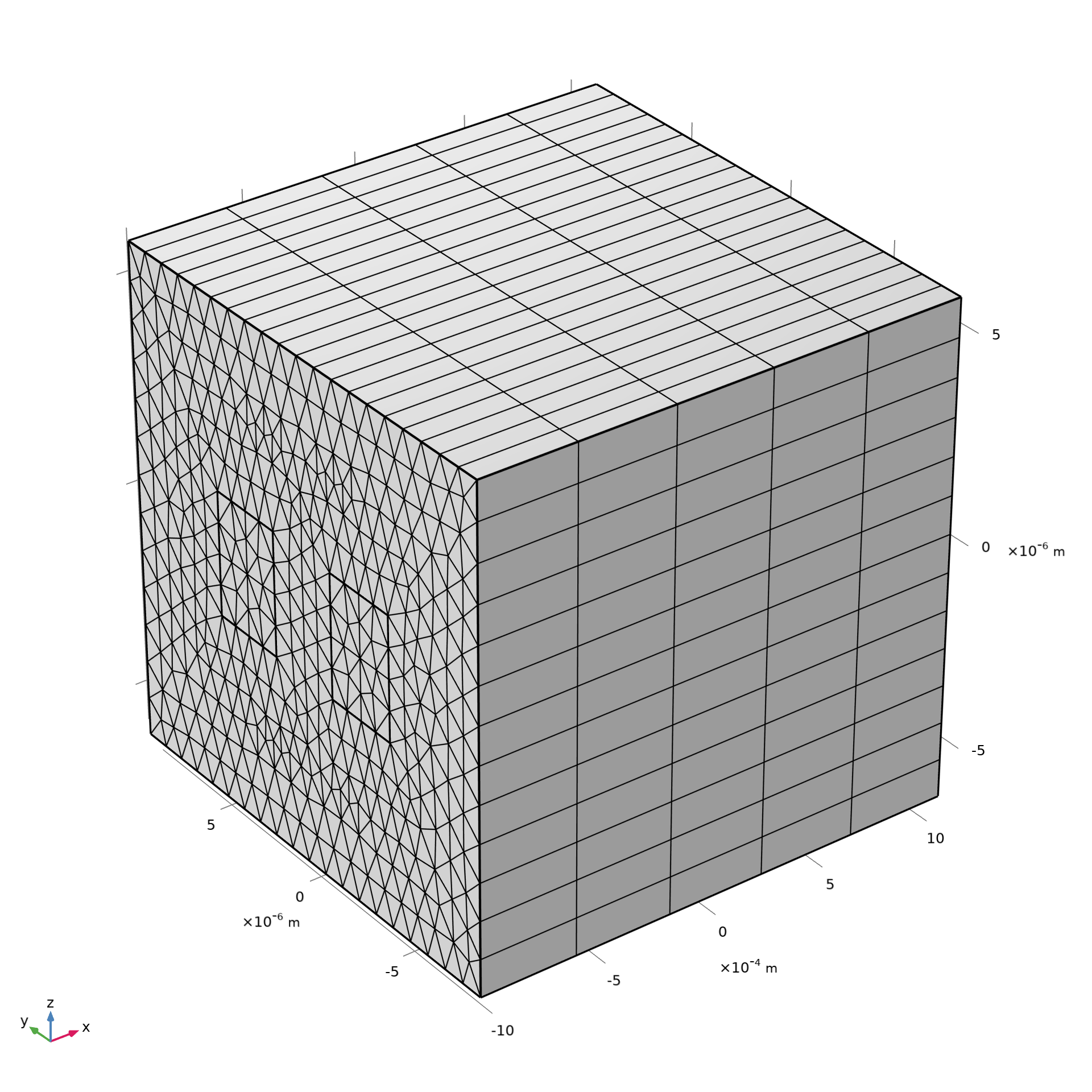
The default tetrahedral mesh generated for the model geometry uses over 120,000 elements, whereas a swept mesh with prism elements contains little over 30,000 elements — a significant difference. There are more elements in the swept mesh than the theory predicts due to the specifics of the topology in this particular geometry. In terms of DOFs, the swept mesh uses 1.3 times less than the default one. The swept mesh also has a higher minimum element quality than the default, unstructured mesh above it.
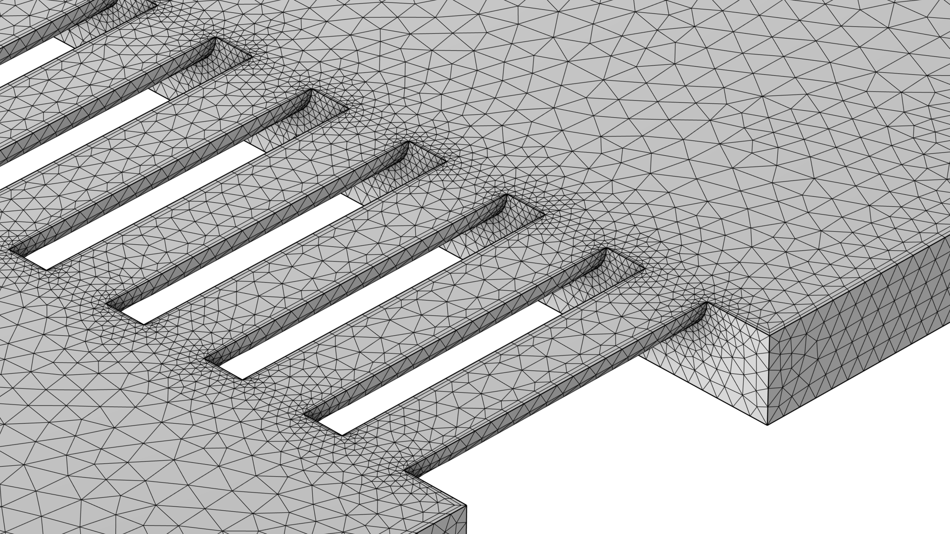
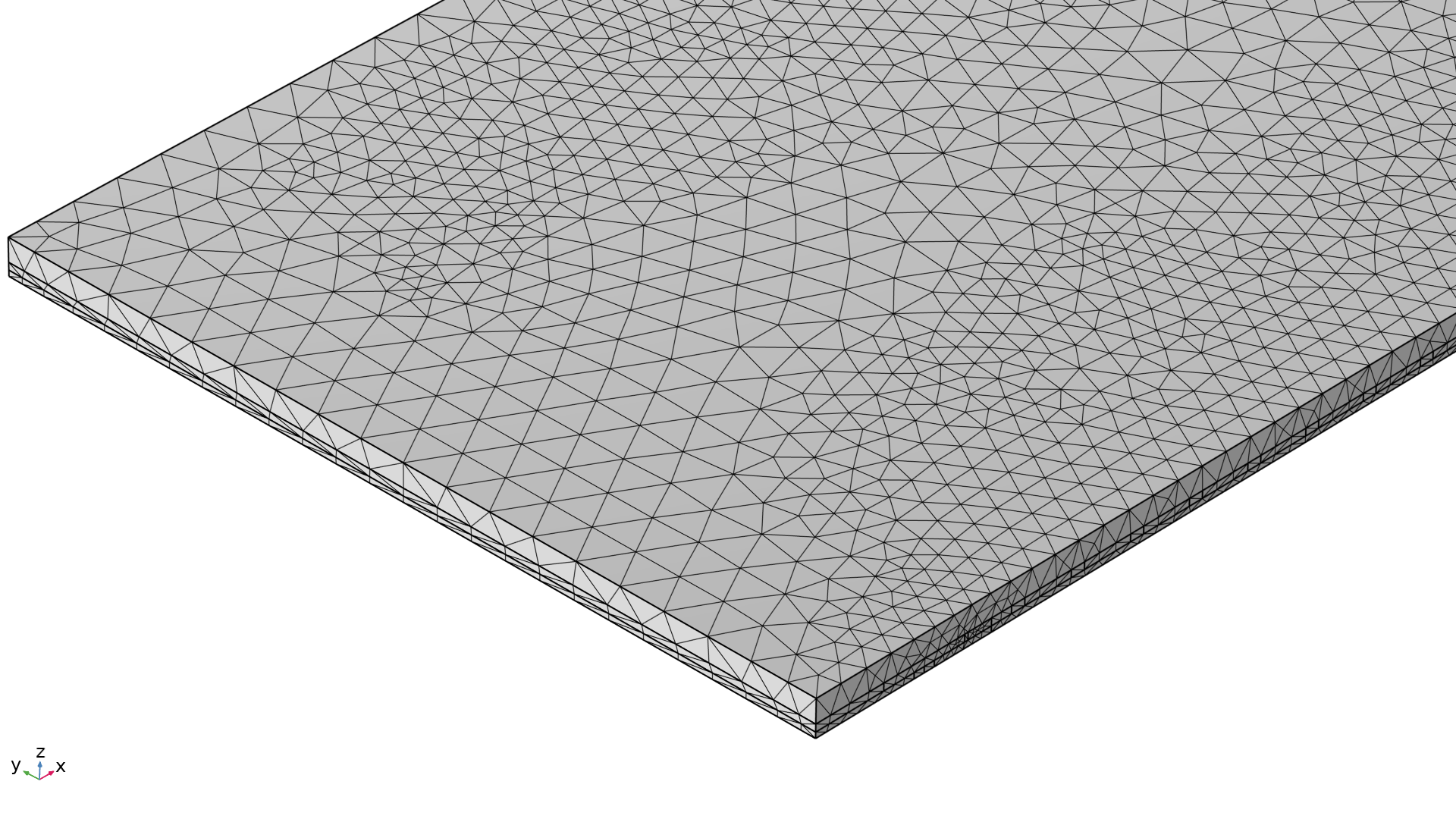 The mesh for the Surface Micromachined Accelerometer model, showing the default tetrahedral mesh.
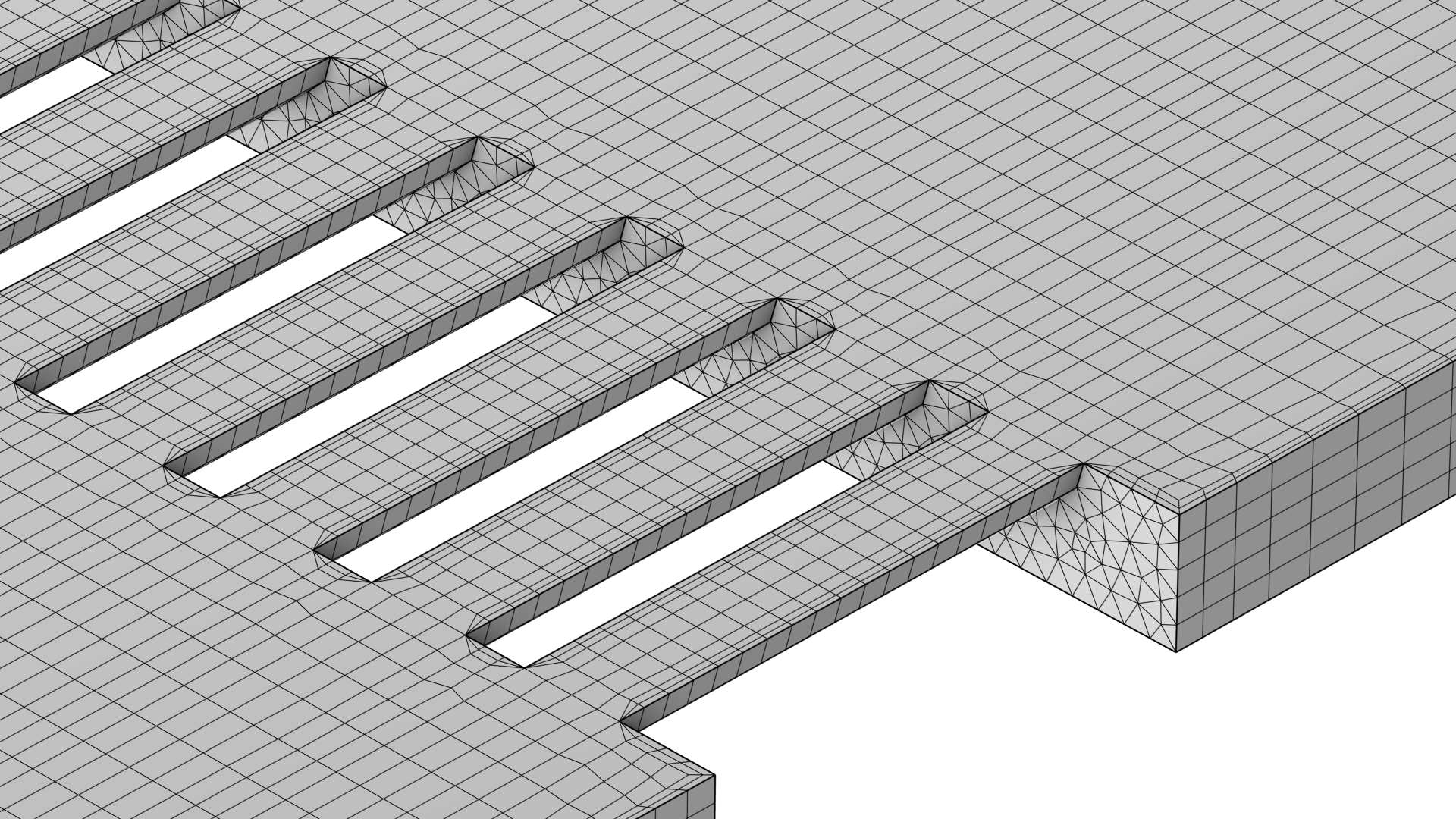
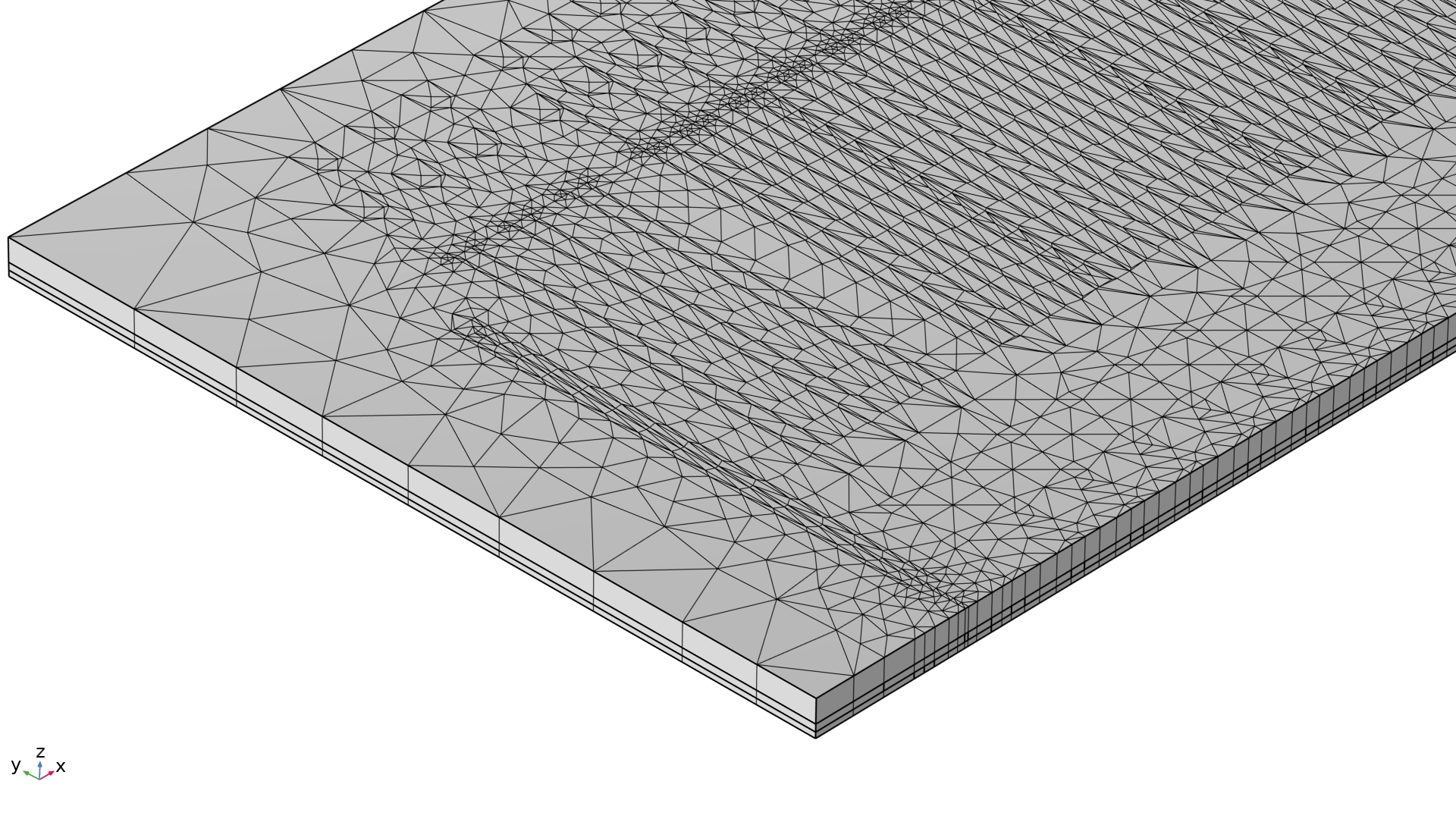 The mesh for the Surface Micromachined Accelerometer model, showing a swept mesh.
The default tetrahedral mesh for the Surface Micromachined Accelerometer tutorial model (left) with the size for the elements set to Normal. The swept mesh for the same geometry (right) contains significantly less elements.
Use Cases
We have presented the three major advantages of swept meshes, which are not physics specific. We will now present concrete examples where those advantages are put to use:
- Slender Structures with High Aspect Ratios
- Solution has a Specific Directionality
- Thin or Narrow Regions Inside Domains
- Resolution of High Gradient in Solution
- Extending the Computational Domain for Better Placement of Boundary Conditions
- Deforming Domains
- Infinite Element Domains and Perfectly Matched Layers
- More Generic Geometries
We expand on each of these specific use cases below.
Slender Structures With High Aspect Ratio
When modeling, you may encounter situations where the geometry in one dimension is significantly larger or smaller than the other two dimensions. This is often the case for integrated circuits and printed circuit boards, which are important in the MEMS industry, or when modeling cables and pipes, whether it be for modeling CFD, solid mechanics, or electromagnetism.
 Geometry of a pouch cell model.
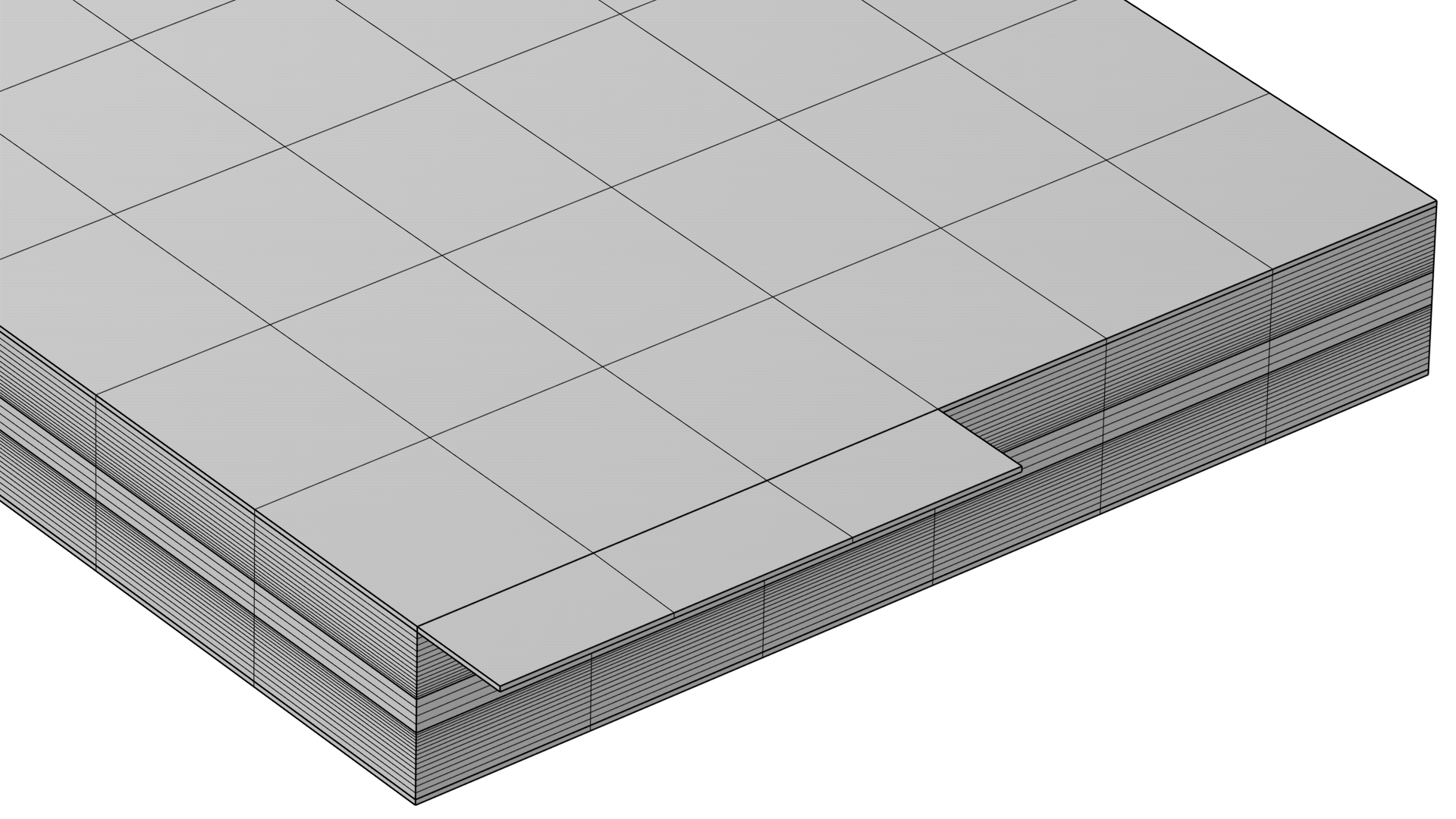 One side of the meshed pouch cell geometry.
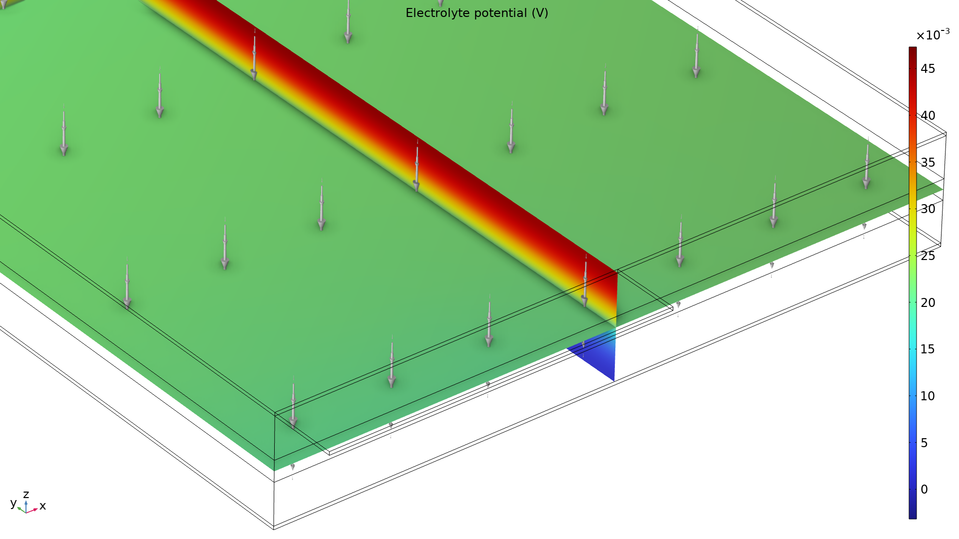 The pouch cell geometry in green, with arrows and a partition down the middle in the Rainbow color table.
The view of one side of the geometry (left) and mesh (center) for a pouch cell tutorial model. The rightmost image shows the electrolyte potential with arrows displaying the electrolyte current density vector. The images are scaled 100 times in the z direction. The thin geometry and the solution call for a higher mesh resolution in the z direction than in the xy-plane.
For a geometry that is slender or contains slender regions, a tetrahedral mesh may be good for modeling some physics phenomena, but not all. Because of this, it can be crucial to be able to generate a swept mesh where the elements are stretched in some direction and still have a good-enough quality.
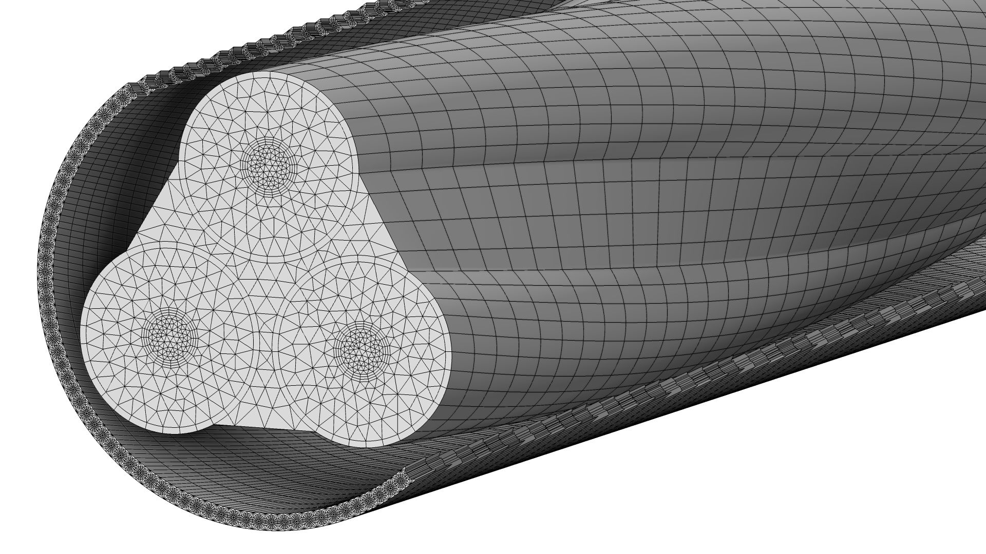
The mesh in the Submarine Cable 7 — Geometry & Mesh 3D tutorial model. The challenge is to find a mesh that resolves the cable geometry and the physics as best as possible, while still keeping the DOF count low enough to have a reasonable solving time.
Solution has a Specific Directionality
For CFD problems, the gradient in the solution is mostly in the direction normal to the flow. Given that the walls do not have a slip condition, a region of high-velocity gradient is forming next to the wall due to viscous effects — this is the so-called boundary layer. This means that the cross section of the swept mesh needs to be well resolved, especially near the walls. In the direction of the flow, the elements can be much coarser, as it is enough to resolve the slow gradient. The boundary layer is resolved by adding a boundary layer mesh along the wall boundaries, while the slow gradient allows for stretched elements in the direction of the flow.
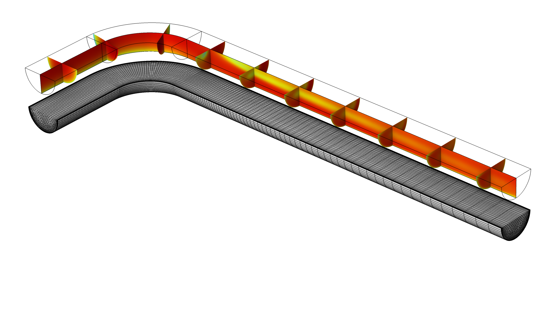 A model of a pipe elbow showing the mesh and velocity gradient.
In the Flow Through a Pipe Elbow tutorial model, the cross section needs to be meshed with a finer mesh size, especially near the walls to resolve the gradient of the solution. The mesh discretization along the flow gradually increases in size as the the gradient of the velocity in this direction becomes smaller. (Each cross section exhibits approximatively the same velocity profile.)
We can use this same strategy to model any physics phenomenon that has a slow gradient in one direction. This typically happens when solving a model with the Electromagnetic Waves, Beam Envelopes interface, which is used when the propagation length is much longer than the wavelength. The mesh does not need to resolve the wave on a wavelength scale, but rather the beating between the two waves. In some cases, only one element is needed along the propagation direction. (For more information, read this blog post.) In the Directional Coupler tutorial model, few mesh elements are needed in the wave propagation direction.
 A cube geometry showing different meshes and elements on three sides.
 The electric field of the Directional Coupler model in the Rainbow color scale.
On the left, the mesh being used for the Boundary Mode Analysis and Frequency Domain studies. Notice the scale; in the x direction, the elements are, in reality, 110 times longer. The bidirectional formulation is used and, in this case, the two wave vectors are codirectional — they point in the same x direction. Since it is expected that the two waves have almost constant amplitudes, the mesh can be very coarse in the propagation direction. The right figure shows the resulting electric field, with a modified scale in the z direction to fit the plot.
Thin or Narrow Regions Inside Domains
Swept meshes can be useful for small details and narrow regions in geometries. To obtain the best possible mesh in these scenarios, you may need to partition the computational domain in order to sweep a mesh in each part separately and also control the size and type of elements in each partitioned domain. This strategy of meshing domains with different settings can be found in our blog post, Best Practices for Meshing Domains with Different Size Settings. The main takeaway is to start sweeping the mesh from the domain where you want to use the smallest mesh size, which is generally either the smallest domain or the one with the steepest gradients in the solution. A typical example is the presence of small channels connecting wider domains in fluid dynamics applications. We know the solution will have a steep gradient in these regions since it may be the place of an accelerating flow.
 A CFD application model with a tetrahedral mesh.
 A CFD application model with a swept mesh.
The default tetrahedral mesh (left) versus a swept mesh (right) in a CFD application with narrow regions. The boundary layers are added as a last step once the domain mesh has been generated.
Resolution of High Gradient in the Solution
In semiconductor models, for example, it is common that the solution gradient has to be well resolved in one direction only. The various physical processes that are involved often require very different length scales. Most of all, doping profiles need to be correctly resolved, as explained in this blog post.
In this bipolar transistor tutorial model, the mesh used is a structured swept mesh where the resolution in the vertical direction is largest around the p-n junctions and near the electrical contacts on the top and bottom surfaces.
The use of swept meshing in semiconductor models is even more crucial, as most models are based on a finite volume method since they inherently conserve current and therefore usually provide the most accurate result for the current density of the charge carriers. For the same mesh, this method requires more DOFs than the finite element method. Given that 3D semiconductor computations can take days to solve, anything to make that process more economical is welcomed and encouraged, of which swept meshing is one. It's use is particularly well suited for these types of problems.
Extending the Computational Domain for Better Placement of Boundary Conditions
Boundary conditions define how the solution connects to the outside world. The interior field will depend on which kind of condition we use, which value we assign to it, and where we place the condition itself. For some models, where to place the boundary conditions is obvious.
We always need to keep in mind that, at the limit of our computational domain, the solution (or its gradient) is imposed. Broadly speaking, when we have convective or propagation terms, we should make sure that the boundary condition is placed far enough so not to influence the solution, as explained in this blog post.
When you need to enlarge the computational domain to place the boundary condition in the appropriate spot, what one usually does is extend the computational domain in a specific direction. Extruded domains are perfect fits for swept meshes considering that you are also expecting the solution field to develop in that specific direction.
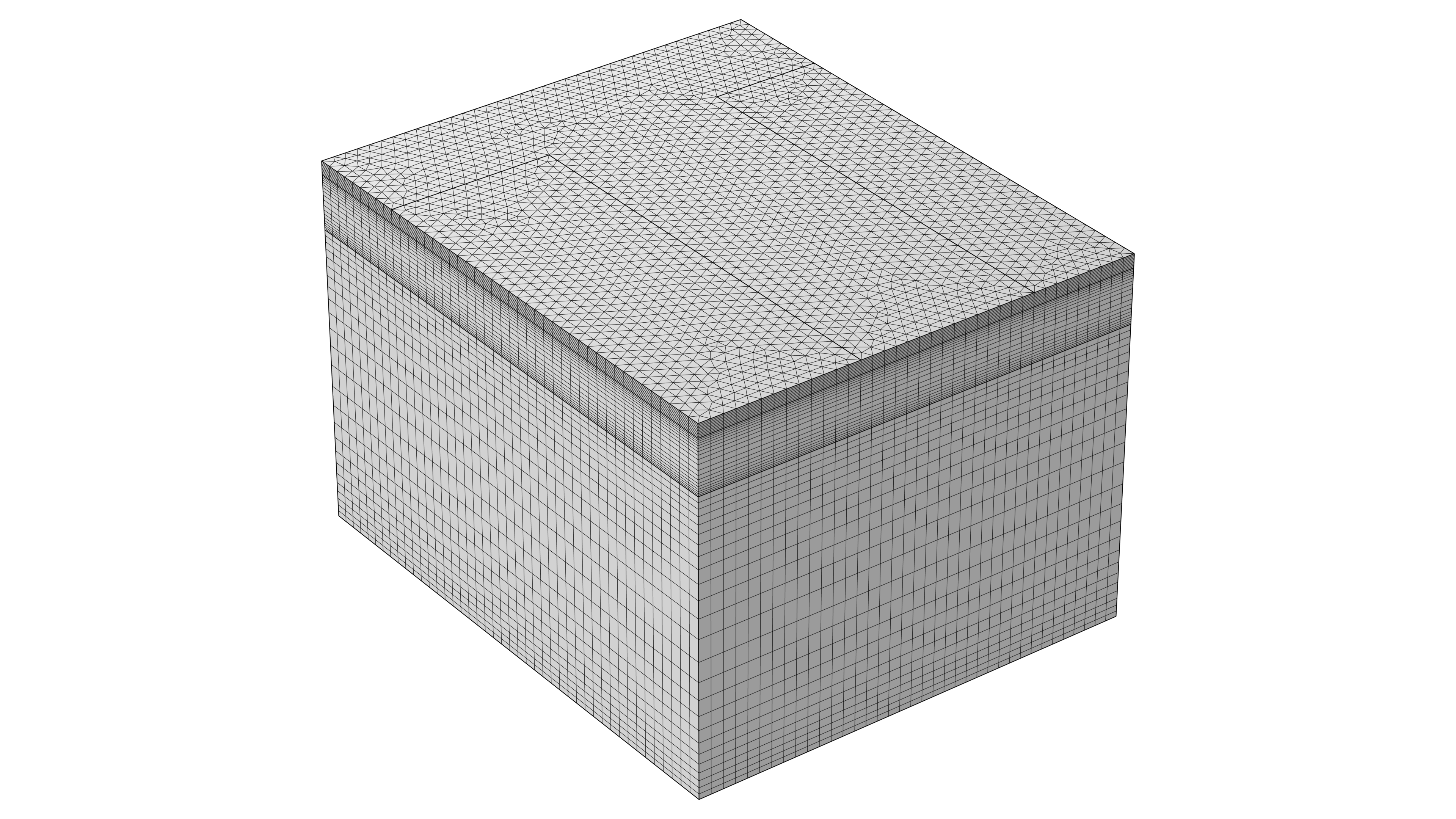
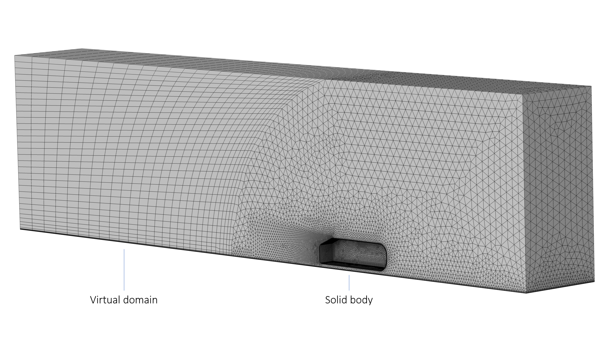 A meshed rectangular model with the virtual domain and solid body labeled.
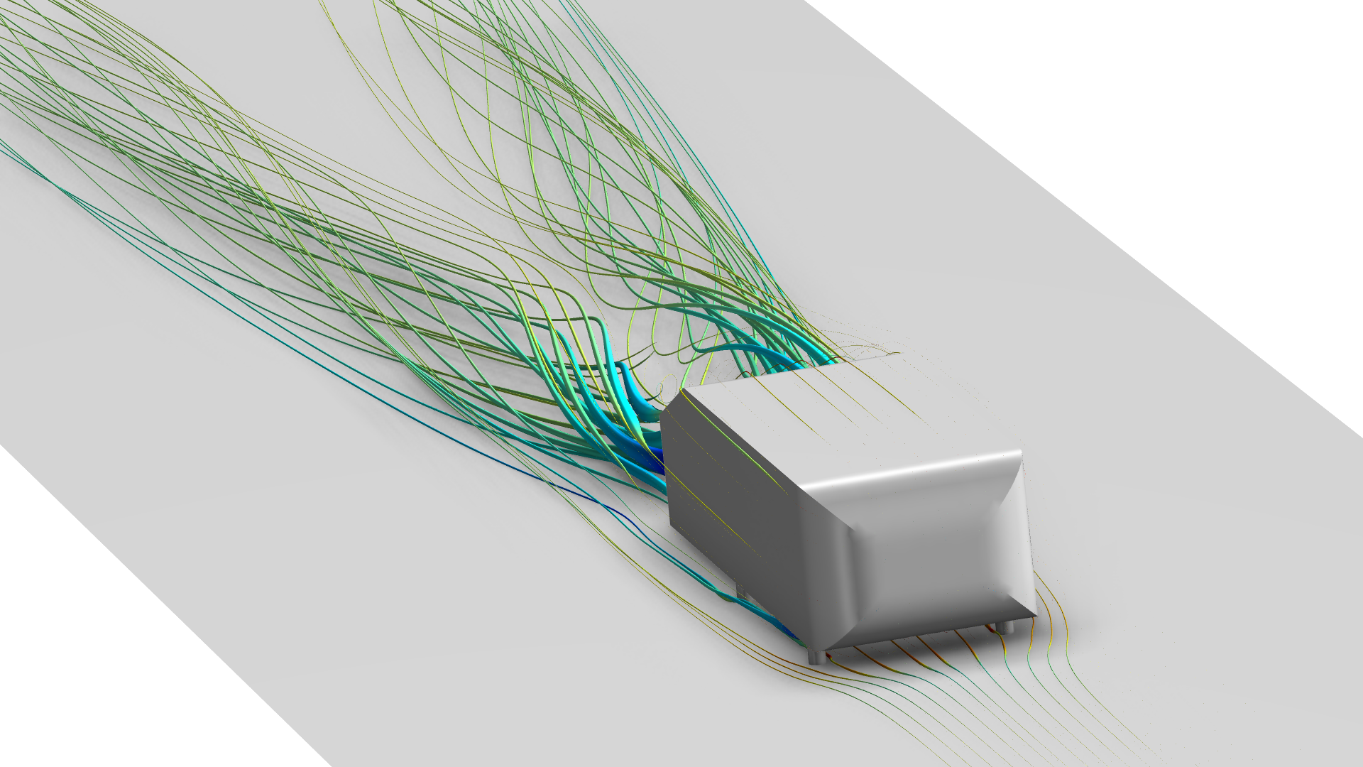 The Ahmed-body streamlines of the airflow around the Ahmed body.
Left: Ahmed body mesh with an extended simulation domain after the body. Right: The wake that the added domain is allowing to form.
Deforming Domains
When deforming a geometry during computations, sliver elements might be generated due to a compression or expansion. As we saw earlier, the element quality of a tetrahedral element is more sensitive to decompression than a prism or hexahedron. If a tetrahedral mesh is used when simulating deformations, it might lead to:
- A need to remesh the deformed configuration one or several times when the elements become too distorted. This results in increased computation time, as the remeshing process takes time and the solution needs to be reinitialized in the new mesh.
- A dense mesh near narrow domain regions, increasing the simulation time by increasing the number of DOFs.
- A risk that the simulation cannot converge due to bad-quality elements.
In the case where you solve for a translation, the direction of compression or expansion can be predicted in advance. This would be the perfect opportunity to use a swept mesh to reduce the need of remeshing. If the geometry is partitioned to allow for a sliding mesh (as described in this blog post), the problem will be more constrained, making the computation even faster and more robust.
In this power switch tutorial model, iron plungers are moved by means of the magnetic attraction exerted by current flowing in the coils surrounding it. In the animation, the magnetic flux density norm is colored in the plunger domains. The air gap (white mesh) between the plunger and the coil is separated from the rest of the air domain (grey mesh) in order to be swept meshed. As the plunger moves toward the lower E-core, it closes the air gap, compressing the swept mesh vertically.
Infinite Element Domains and Perfectly Matched Layers
Some models need a region of infinite extent. They can be modeled as either infinite element domains, perfectly matched layers (PML), or absorbing layers. For PMLs and absorbing layers, it is important that the mesh matches the coordinate stretching direction, that is, the direction of absorption. The reason for this is that these virtual domains are numerically stretched out toward infinity, so we must take into account that the mesh elements will be virtually elongated. The fact that swept mesh elements keep a good quality at high aspect ratio is consequently the key, again!
If an infinite element domain or PML is used by the physics, a swept mesh will automatically be generated by the physics-controlled mesh.
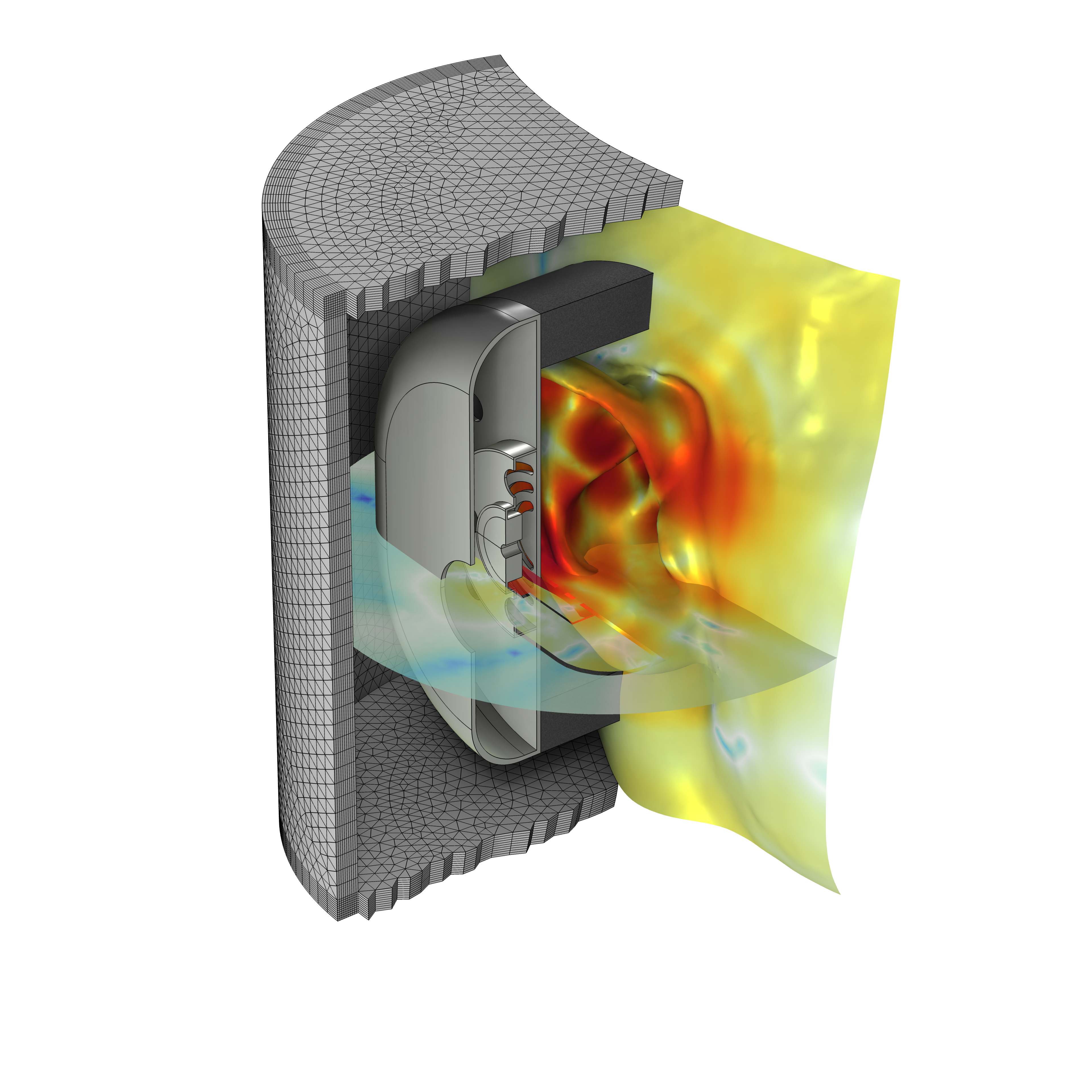
In the Headphone on an Artificial Ear tutorial model, cylindrical PMLs are used around the geometry, which are meshed with a swept mesh (represented partially in the image in order to visualize the interior geometry). The resulting sound pressure level at 20 kHz is depicted on the manikin and slice of the air domain.
More Generic Geometries
What about domains of a more generic shape? For those, a swept mesh can still be used. Recall the first advantage of swept meshes: the swept mesh will require about half as much of DOFs compared to a tetrahedral mesh. However, domains of more general shape may require some additional work to be made sweepable. We will look further into this later in the course.
It is not always possible to use a swept mesh for the whole geometry. Nonetheless, you can get the best of both worlds by combining a swept and a tetrahedral mesh by generating a swept mesh in as much of the geometry as possible, and then meshing the rest with a tetrahedral mesh.
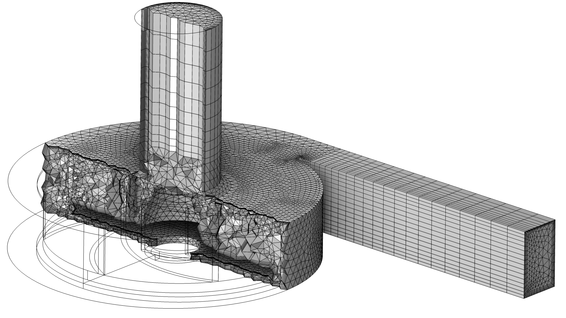 The Centrifugal Pump model with various mesh elements.
A tetrahedral mesh is combined with a swept mesh in the Centrifugal Pump tutorial model.
Alternatives to Generating Meshes for Thin Domains
We have discussed at great length the opportunities for using swept meshes to discretize the model geometry, however, there are some times in which an alternative strategy might be optimal. This is especially in cases that involve working with thin and/or slender geometries. COMSOL Multiphysics® has many specialized physics interfaces as well as physics feature nodes that enable you to more efficiently model thin regions with high aspect ratios. There are also options for modeling such regions as surfaces or edges instead of as 3D domains. You can learn about this functionality and the corresponding features in COMSOL Multiphysics® in the following blog posts:
- Coupling Structural Mechanics Interfaces
- Analyze Thin Structures Using Up and Down Operators
- Modeling Piezoelectricity: Which Module to Use?
The physics interfaces and boundary conditions mentioned in these blog posts enable you to easily address thin domains or layers in geometry. In addition, you can see what features are available for CFD simulations by referencing the fluid flow specification chart.
Further Learning
In this article, we focused on understanding what swept meshes are and when you should use them, as well as when to use them in combination with a tetrahedral mesh. Several examples were showcased in this article, and we encourage you to use the provided links to explore the models further. Additionally, in the software under the Application Libraries you can search @tag:swe to find any tutorial model examples that use swept meshing for the model geometry. By navigating to the appropriate application area you are interested in, you can find relevant examples and understand the logic behind why a swept mesh was used or was incorporated into a mesh as well as how it was implemented.
请提交与此页面相关的反馈,或点击此处联系技术支持。