使用偏微分方程(PDE)接口建模:全局常微分和微分代数方程接口
在 COMSOL Multiphysics® 中使用偏微分方程(PDE)接口建模系列课程的第 6 部分,我们将介绍如何求解与时间相关的常微分方程(ODE)和微分代数方程(DAE)。这些方程与空间维度无关,因此也与网格或几何结构无关。为此,您可以使用 全局常微分和微分代数方程 接口,这类方程也称为初始值问题。我们还将讨论线性和非线性方程,包括方程组。
目录
全局常微分和微分代数方程
与使用偏微分方程建模一样,如果您有一个需要将常微分方程作为初始值问题建模的普通应用,您可能会想在 COMSOL 的某个附加产品中找到一个容易使用的内置接口。如果要了解哪些内置接口可供使用,请打开一个新模型,并在 选择空间维度 窗口中选择 0D 选项,此选项常用于表示没有任何空间依赖性的初始值问题。
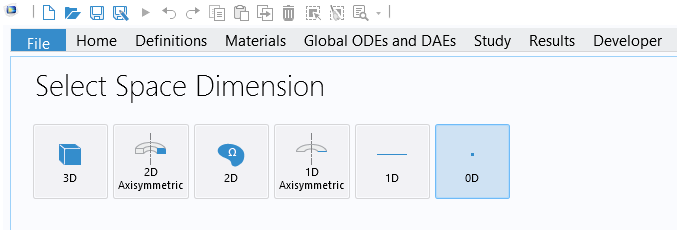
0D 选项。
在 选择物理场 界面中,您将看到可用的 0D 接口列表,如下图所示。要查看这些接口的完整列表,您需要访问不同的附加产品。
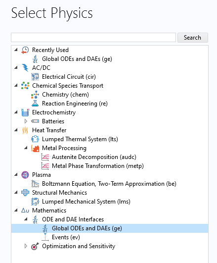
内置的 0D 物理场接口,用于对常微分方程的初始值问题进行建模。
在上图中,突出显示了通用的 全局常微分和微分代数方程 接口。如果您想求解自己的常微分方程或常微分方程组,应选择此接口。如果您有一个微分代数方程组,即微分方程与代数方程的混合方程,也可以使用该接口求解。
求解含约束的质量-弹簧-阻尼系统的常微分方程
我们先来看一个简单的例子,了解如何求解下面这个经典的受迫质量-弹簧-阻尼系统的二阶初始值问题:

这种微分方程的书写方式使用的是 莱布尼兹记号法。
我们可以将其简写成

这就是所谓的 拉格朗日记号法。
还有一种方法是牛顿记号法:

在此,我们将使用拉格朗日记号法。
受迫质量-弹簧-阻尼系统可以通过含有时间相关变量  的方程来表示,表示质量为
  的点从平衡位置的位移。系数
  代表阻尼,
代表阻尼, 是弹簧常数。等号右边的函数
  代表外部约束函数。二阶常微分方程有两个初始条件:


有关质量-弹簧-阻尼模型的更多信息,请参见 https://en.wikipedia.org/wiki/Mass-spring-damper_model。
我们将模拟如下参数所代表的质量-弹簧-阻尼系统:


假设您选择了 全局常微分和微分代数方程 接口,那么在模型向导的最后一步,请选择 瞬态 研究,如下图所示。
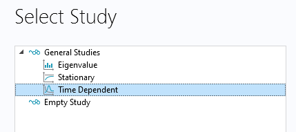
在求解初始值问题时,需要进行 瞬态 研究。
这样就可以使用 全局方程 接口了,如下图所示。
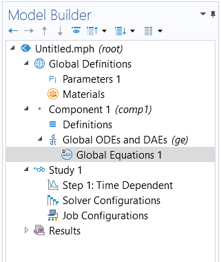
常微分方程的数学接口称为 全局方程。
在定义方程之前,创建以下全局参数:
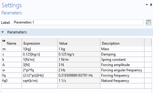
质量-弹簧-阻尼系统使用的参数。
在用户接口中,可以使用语法 ut 和 utt 分别表示一阶和二阶导数。
全局方程 接口要求我们在表格中输入方程:

为了使等式符合用户接口所需的格式,我们将等式稍作改写:

这样,我们就有:

式中使用的符号在 COMSOL® 中是依照惯例选择的,即,作用在系统上的外部(广义)力应以正号写入方程。
请注意,这个接口也接受隐式非线性常微分方程。正如函数  的形式所指示的,可以用一个数学表达式来定义一个常微分方程,其中涉及解变量、它的一阶和二阶时间导数,以及对时间变量 t 的显式依赖关系。
在 全局方程 接口,现在可以输入以下内容:
- 名称:
u - 方程 f(u,ut,utt,t):
A*cos(w*t)-m*utt-c*ut-k*u - 初始值:
u(0)=2 - 初始值:
u'(0)=0 - 因变量,位移:
m - 源项量,力:
N
在下图中,已将这些设置输入用户界面:
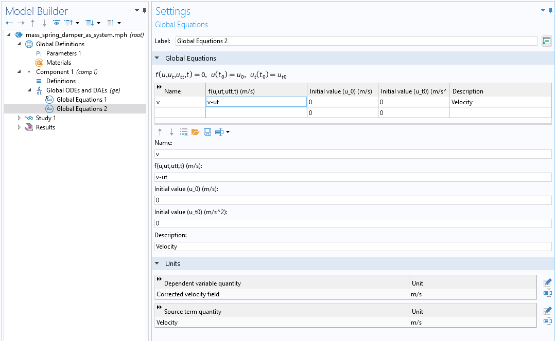
质量-弹簧-阻尼常微分方程的 全局方程 设置。
下一步是定义要求解的时间序列。
在模型开发器中,选择 研究 > 步骤 1:瞬态 节点。将 输出时步 表达式中的最后时间改为 50。语法 range(0,0.1,50) 表示求解器将以 0.1 s 为间隔从 0 s 到 50 s 输出结果。算法采用自适应,会根据方程的行为和设定的容差,采取比指定的 输出时步 更多或更少的时步。
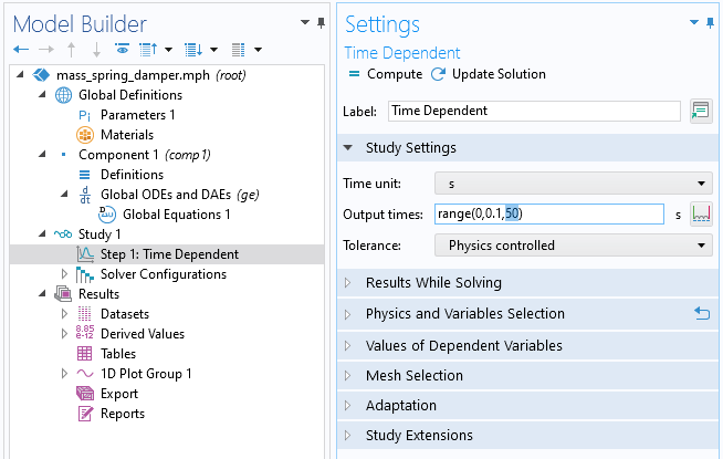
输出时步 设置为在 0s 至 50s 之间求解。
点击 计算 求解。默认曲线图显示的是求解结果与时间的关系。
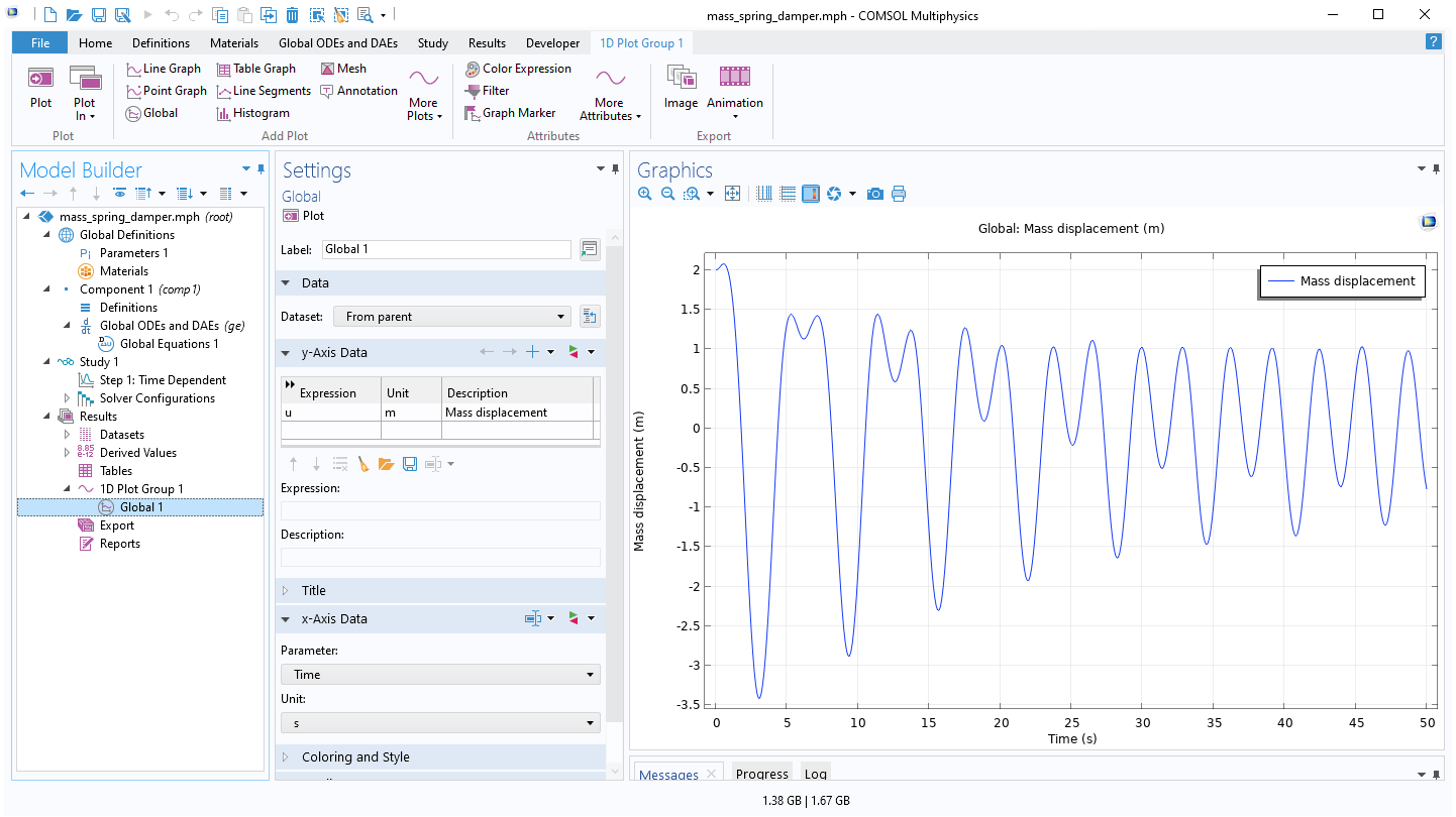 The Model Builder with a Global plot selected, the corresponding settings, and the Graphics window showing the mass displacement.
0 s 至 50 s 之间的质量-弹簧-阻尼常微分方程的解。
The Model Builder with a Global plot selected, the corresponding settings, and the Graphics window showing the mass displacement.
0 s 至 50 s 之间的质量-弹簧-阻尼常微分方程的解。
要了解所获解的精确度,可以减小容差。如下图所示,在 瞬态设置 窗口中,将 容差 选项从 物理场控制 更改为 用户控制,并将 相对容差 设为 0.0001(或 1e-4)。

瞬态 研究的 相对容差 设置。
如下图所示,解略有变化。
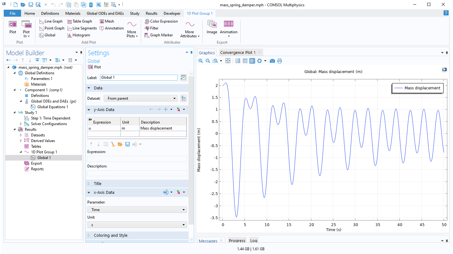 The Model Builder with a Global plot selected, the corresponding Settings window, and the Graphics window showing the updated mass displacement.
质量-弹簧-阻尼微分方程的解,具有较小的求解器容差。
The Model Builder with a Global plot selected, the corresponding Settings window, and the Graphics window showing the updated mass displacement.
质量-弹簧-阻尼微分方程的解,具有较小的求解器容差。
您甚至可以对不同的容差值创建参数扫描,如下图所示。
 The Model Builder with a Global plot selected, the corresponding settings, and the Graphics window showing different mass displacement results.
质量-弹簧-阻尼器常微分方程的逐渐减小求解器容差的扫描结果。
The Model Builder with a Global plot selected, the corresponding settings, and the Graphics window showing different mass displacement results.
质量-弹簧-阻尼器常微分方程的逐渐减小求解器容差的扫描结果。
请注意,此示例的相关文件可在本页面右侧下载。
我们可能还对解的频率内容感兴趣,可以尝试显示原始质量-弹簧-阻尼器模型(无容差扫描)的频谱,在 全局绘图设置 窗口中将 x 轴数据 部分的 参数 选项更改为离散傅里叶变换,然后将 显示 选项更改为 频谱。如下图所示:
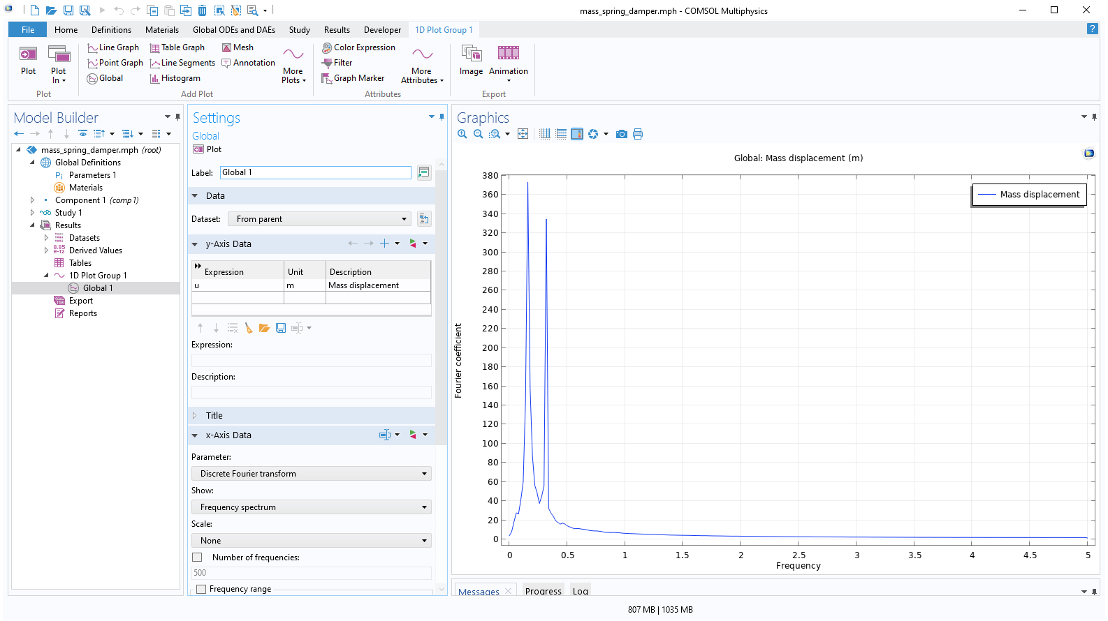 The Model Builder with a Global plot selected, the corresponding Settings window, and the Graphics window showing frequency versus Fourier coefficient.
质量-弹簧-阻尼模型的频谱。
The Model Builder with a Global plot selected, the corresponding Settings window, and the Graphics window showing frequency versus Fourier coefficient.
质量-弹簧-阻尼模型的频谱。
点击 图形 工具栏上的 x 轴对数刻度 和 y 轴对数刻度 按钮,可以绘制对数(log)刻度的坐标轴图。这样就可以绘制出以下图形:
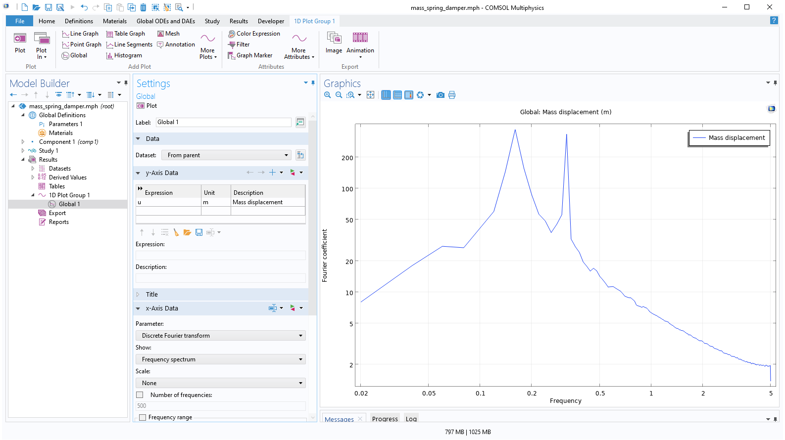 The Model Builder with a Global plot selected, the corresponding settings, and the Graphics window, with the graph plotted with a log scale.
质量-弹簧-阻尼模型的频谱,用对数刻度绘制。
The Model Builder with a Global plot selected, the corresponding settings, and the Graphics window, with the graph plotted with a log scale.
质量-弹簧-阻尼模型的频谱,用对数刻度绘制。
我们可以看到在 0.16 Hz 和 0.32 Hz 处有两个频率峰值。请注意,如果求解的时间周期更长,就会出现与约束频率相对应的尖峰,因为约束频率决定了稳态周期解。
求解常微分方程组
全局常微分和微分代数方程_ 接口还可用于求解常微分方程组。在化学工程中,通常需要求解包含数百个(有时甚至数千个)方程的常微分方程系统。化学反应工程模块具有输入此类系统的专门建模功能。在电气工程中,对电路进行建模时也可能会遇到大型常微分方程组,这可以用 电路 接口求解,包括 AC/DC 模块在内的多个附加产品都内置 电路 接口。
这里,我们将研究一个简单的二变量系统:质量-弹簧-阻尼方程系统。通过引入点质量的速度  作为新的自由度,

可以将二阶质量-弹簧-阻尼方程重写为两个一阶方程组成的方程组:


我们可以通过多种方式在用户界面中输入这个系统。如下图所示,我们只需在 全局方程 接口的第二行添加速度方程即可。
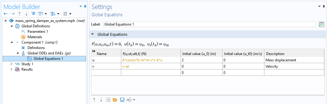 The Model Builder with the Global Equations interface selected and the corresponding Settings window.
微分方程组等价于标量质量-弹簧-阻尼微分方程。
The Model Builder with the Global Equations interface selected and the corresponding Settings window.
微分方程组等价于标量质量-弹簧-阻尼微分方程。
这个方程组可以正确求解;但是,如果我们这样做,就会遇到处理单位的问题。方程的黄橙色表示当前单位不一致。如果想要单位一致,就需要添加第二个 全局方程 接口,并将 因变量物理量 和 源项物理量 的单位更改为 m/s。如下图所示。
用于将二阶质量-弹簧-阻尼微分方程重写为一阶微分方程组的第二个速度变量微分方程。
求解这个一阶方程组的解法与求解标量二阶方程的解法相同。
我们还可以在相平面上绘制解,即在一个轴上绘制位移 u,在另一个轴上绘制速度 v。这是一个二维绘图,为此需要首先创建一个二维数据集。右键单击 结果 > 数据集 节点,在 更多二维数据集 下选择 二维栅格,如下图所示。
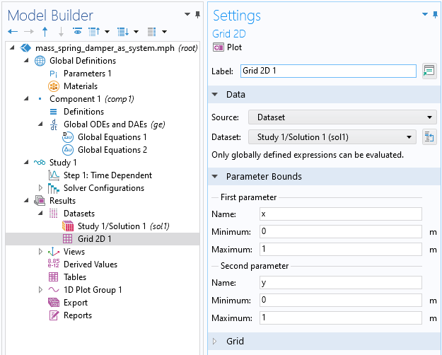
用于绘制相位平面图的 二维栅格 数据集。
不需要更改 二维栅格 数据集的设置,因为我们将绘制具有全局变量范围的量。
接下来,右键单击 结果 节点并选择 二维绘图组。然后,右键单击该 二维绘图组,选择 更多绘图 下的 点轨迹。在 点轨迹设置 窗口中,分别为 x 表达式 和 y 表达式 输入 u 和 v,如下图所示。
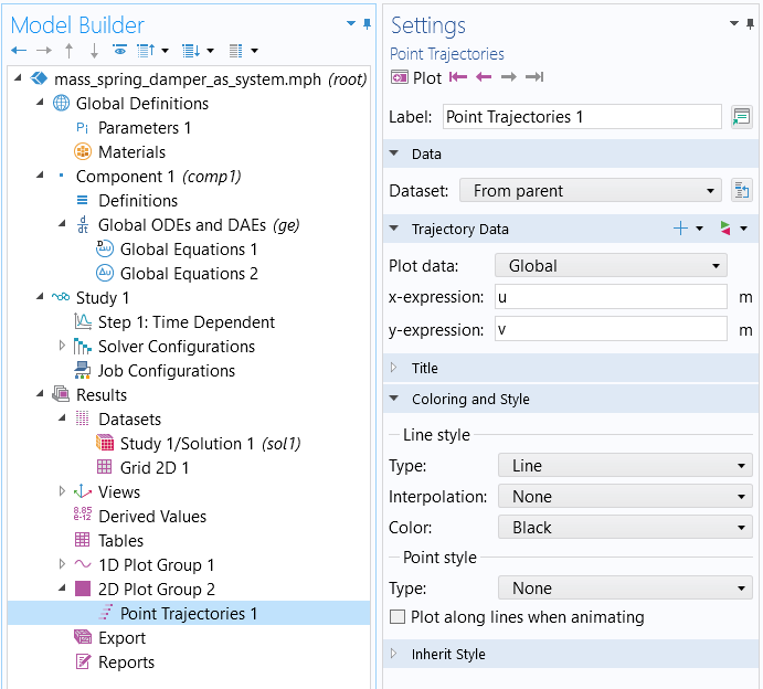
用于绘制相位平面图的 点轨迹 设置。
然后,取消勾选 二维绘图组 设置中的 绘图数据集的边 复选框,如下图所示。

为 点轨迹 绘图清除绘图数据集边。
现在,我们可以得到以下相平面图:
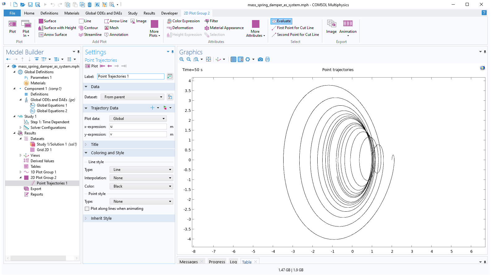 The Model Builder with the Point Trajectories plot selected, the corresponding settings showing the plot data, and the Graphics window showing the plot.
质量-弹簧-阻尼微分方程的相平面图。
The Model Builder with the Point Trajectories plot selected, the corresponding settings showing the plot data, and the Graphics window showing the plot.
质量-弹簧-阻尼微分方程的相平面图。
如果我们对常微分方程进行长达 200 s 的求解,而不是目前的 50 s,能更好地了解结果的行为。
将 输出时步 设置改为 range(0,0.01,200) 并进行计算。结果如下:
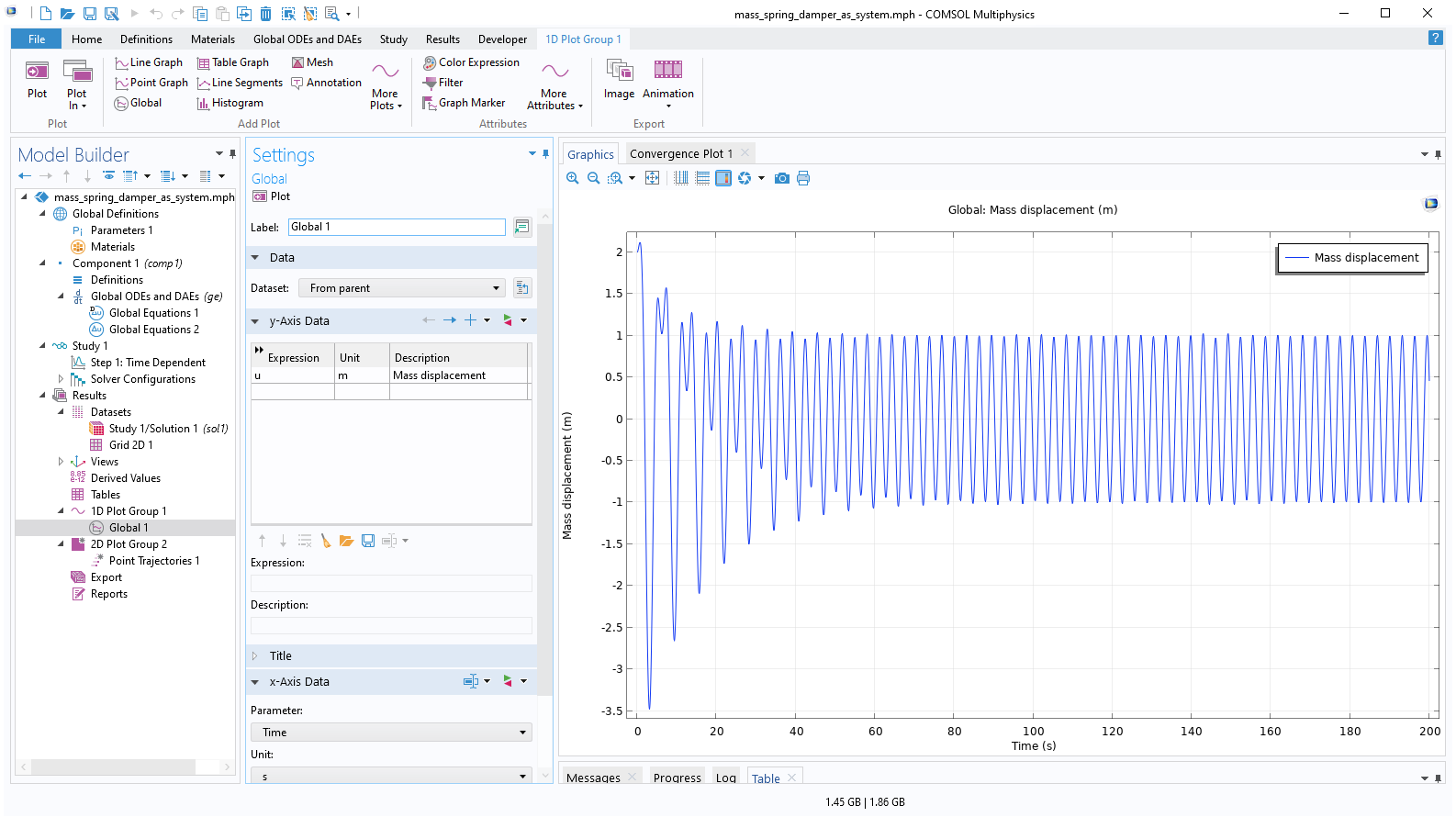 The Model Builder with the Global plot selected, the Settings window with the y-Axis Data section expanded, and the Graphics window showing the mass displacement.
解稳定为正弦波形式,由约束函数的频率决定。对于 c=0.125[kg/s],相应的相平面图如下所示:
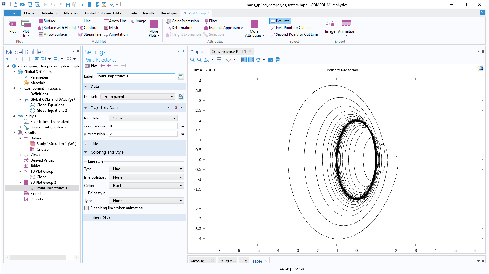 The Model Builder with Point Trajectories selected, the corresponding settings, and the Graphics window with the phase-plane plot.
相位平面图中较暗的区域反映了稳定的解轨迹。
请注意,您也可以通过在 点轨迹 图中输入 ut 来代替 v 来为之前的标量质量-弹簧-阻尼方程生成相平面图。然而,变量 ut 将使用比 u 更低阶的近似值来表示,因此如果我们使用因变量 u 和 v 这种具有相同离散阶数的系统,相平面图看起来会更平滑。
求解非线性常微分方程组
全局常微分和微分代数方程 接口不仅限于求解如质量-弹簧-阻尼系统这样的线性方程,我们几乎可以在方程中输入任何类型的非线性。质量-弹簧-阻尼系统方程的经典非线性扩展是添加一个非线性增益或阻尼项,如下所示:

式中,我们改变了阻尼系数的符号,并将其乘以一个系数  。如果
。如果  较小,则该系数会导致增益;如果 较大,则会导致阻尼。这样,方程就在阻尼和增益之间产生了有趣的相互作用。这一方程已被广泛研究,并被称为 范德波尔振荡器,常用于模拟真空管的振荡。不过,在示例中,我们将把范德波尔方程作为质量-弹簧-阻尼系统的延续,尽管其物理解释并不直接相关。
要输入这个方程,可以修改二阶质量-弹簧-阻尼方程或一阶方程组。在此,我们将修改一阶方程组,如下所示

下图是其中的第一个等式,使用的符号惯例与前面的例子相同。
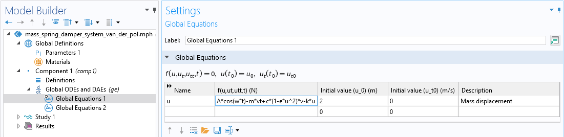 A close-up of the Model Builder with the Global Equations interface selected and a close-up of the Global Equations table in the Settings window.
在 全局方程 接口输入的范德波尔振荡器微分方程。
系数 e 用于生成一致的单位,其定义如下图所示:
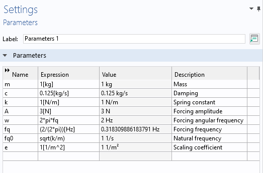
范德尔波尔振荡器微分方程的参数。
将 输出时步 设置为 范围(0,0.01,200) 进行求解,可以得到以下解:
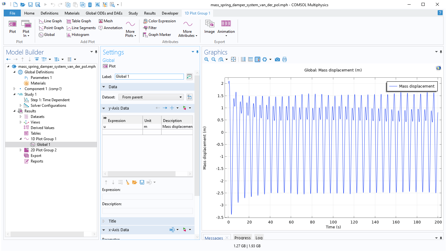 The Model Builder with the Global plot selected, the settings, and the Graphics window showing the solution.
范德尔波尔振荡器微分方程的解。
以及相平面图,如下图所示:
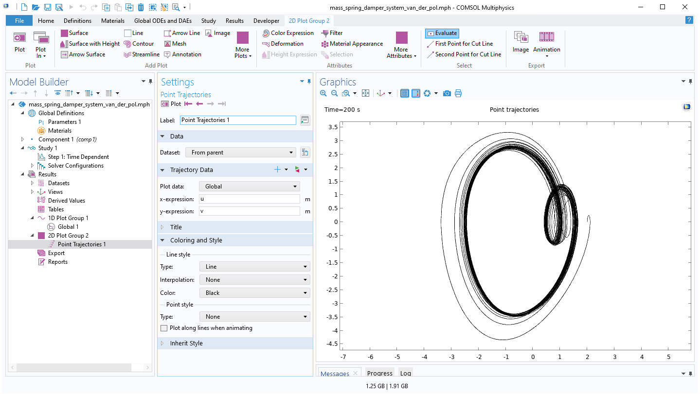 The Model Builder with the Point Trajectories plot selected, the corresponding Settings window, and the Graphics window showing the van der Pol oscillator phase plot.
范德尔波尔振荡器微分方程的相图。
图中颜色较深的部分表示解具有 极限周期。对于时域解来说,这是因为它接近极限周期解。然而,这种极限波形并不是正弦波,而是一种更为复杂的行为。如下图所示,通过放大时域图中的最后几个周期,可以更清楚地看到它的形状:
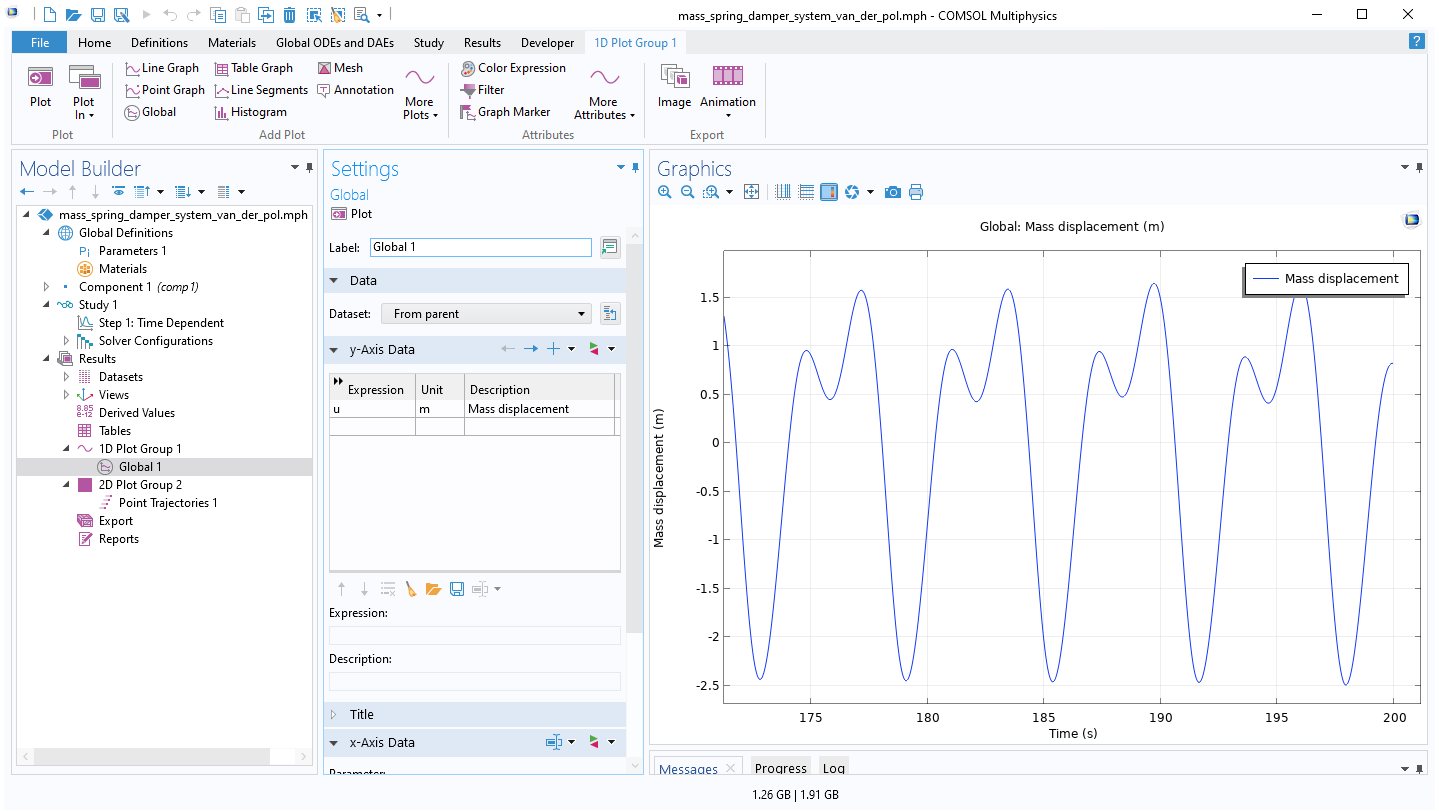 The Model Builder with the Global plot selected, the plot settings, and the Graphics window with the plot zoomed in.
范德尔波尔振荡器微分方程解的放大图。
通过改变阻尼(或增益)系数 c 的值,可以得到其他波形。请注意,方程的非线性也会使频域漂移。下图显示了 c=10[kg/s] 时的波形。
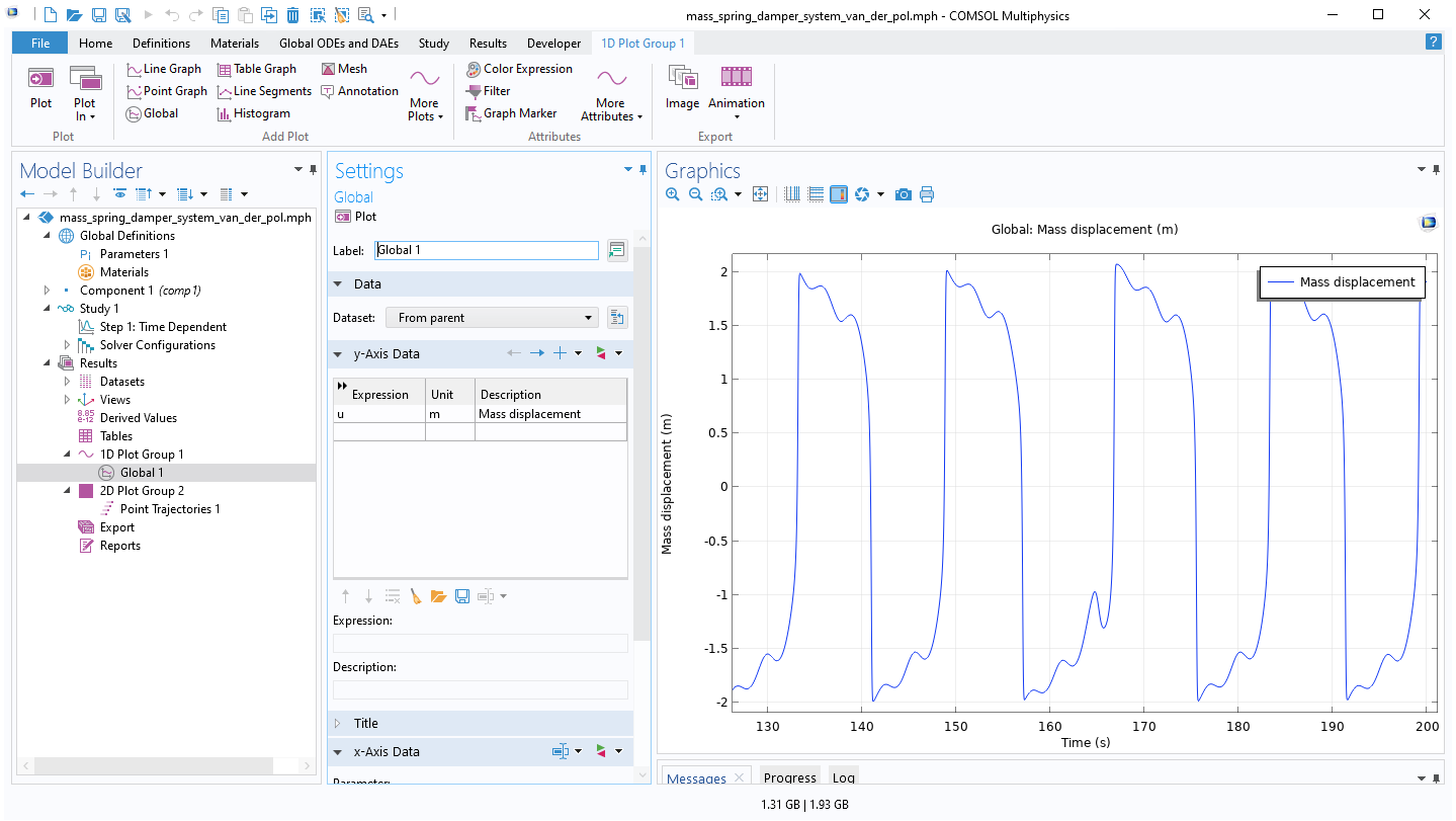 The Model Builder with the Global plot selected, the Global Settings window, and the Graphics window showing the new mass displacement waveform.
不同阻尼系数下范德尔波尔振荡器微分方程的解。
这种波形的频谱比线性质量弹簧阻尼系统复杂得多,如下图所示,绘图采用了对数刻度:
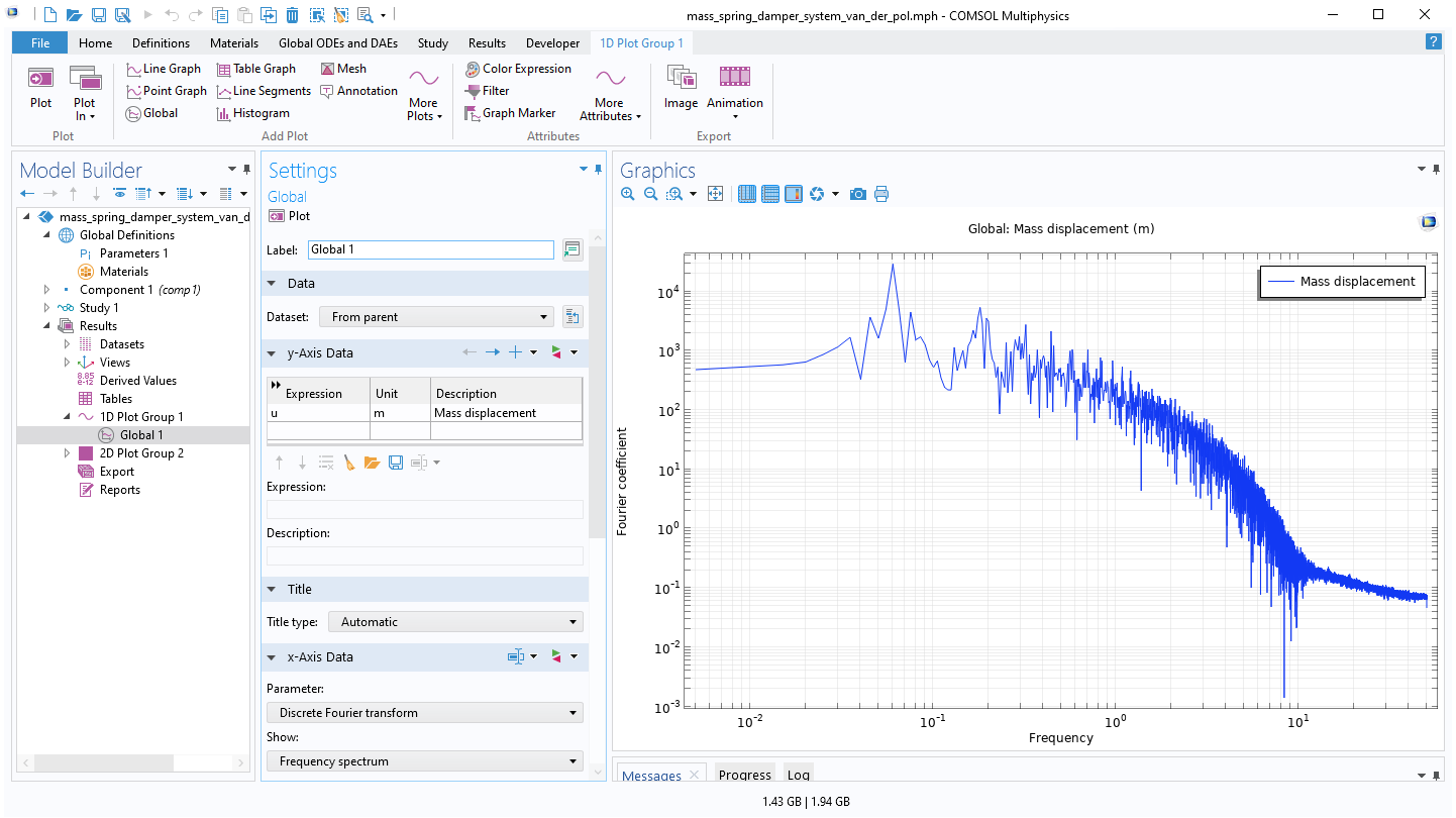 The Model Builder with the Global plot selected, the corresponding Settings window, and the Graphics window showing the frequency spectrum become more complex.
范德波尔振荡器微分方程解的频谱。
绘制相图
许多教科书都有无约束范德尔波尔振荡器的相图:


首先重排该等式,就能得到一个用于绘制相图的表达式:


用 x 坐标表示 u,y 坐标表示 v,可以得到相图。为了得到我们想要的箭头图,可以设置:
 为 x 的分量
和
 为 y 分量
使用坐标为 x 和 y 而不是 u 和 v 的 二维栅格 数据集来绘制这个矢量场,这意味着实际使用的矢量场表达式为
x 分量: y
y 分量: (c*(1-e*x^2)*y-k*x)/m
下图显示了 c=1[kg/s] 时的相图和初始条件 (u, v) = (-3, -3) 时的轨迹。
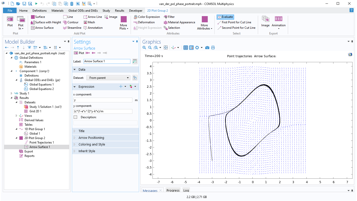 The Model Builder with the Arrow Surface plot selected, the plot settings, and the Graphics window showing the phase portrait of the van der Pol oscillator solution.
范德波尔振荡器解的相图。
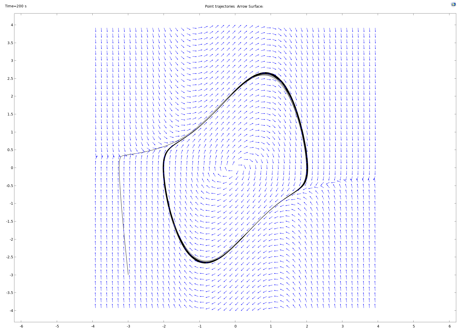 A close-up view of the phase portrait of the van der Pol oscillator solution.
范德波尔振荡器解的相放大图。
相应的文件可在本文随附的可供下载参考文件中找到。
微分代数方程组
在本系列课程的第 10 部分中,我们介绍了与时间相关的焦耳热模型如何成为微分代数方程组的一种形式,因为其中一个方程没有时间导数。同样,全局常微分和微分代数方程 接口也可以求解微分代数方程组。
例如,下面的方程组在第一个等式中有时间导数,但在第二个等式中没有:


下图显示了该微分代数方程组的用户接口:
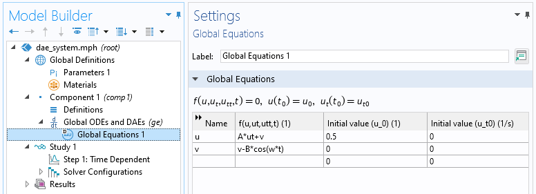
在 全局方程 接口输入的微分代数方程组。
请注意,由于没有时间导数,因此第二个方程的 初始值 并不重要。
下图显示了该方程组的解:
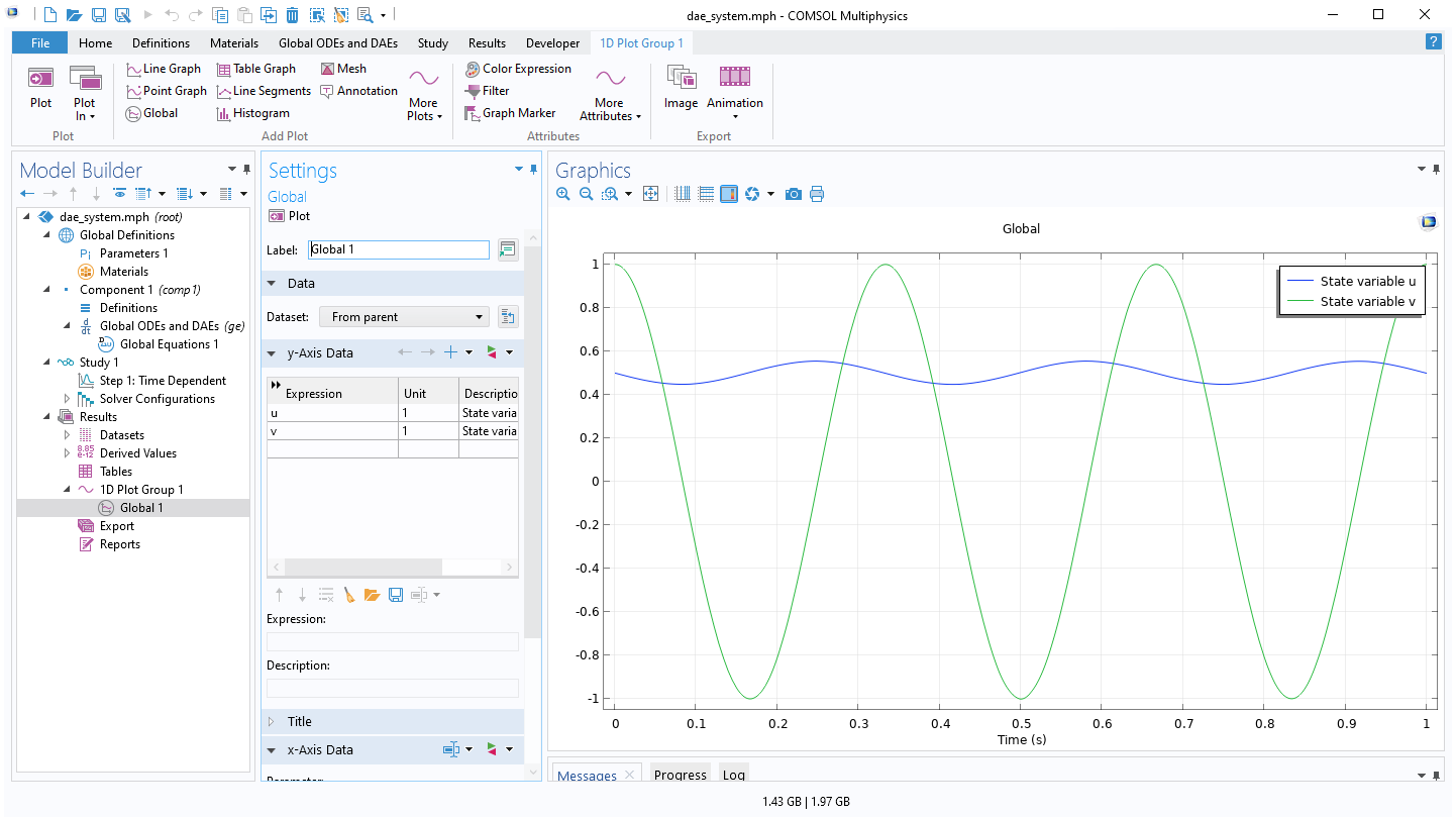 The Model Builder with the Global plot selected, the settings, and the Graphics window showing the state variable u in blue and the state variable v in green.
微分代数方程组的解。
本例中使用的参数如下图所示:
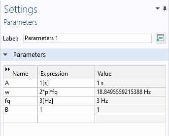
微分代数方程组的参数。
耦合偏微分方程模型与常微分方程
您可以将一个或多个 全局方程 接口添加到现有的物理场接口中,以创建自定义的常微分方程耦合。下图显示了添加到 电流 接口的 全局方程 接口:
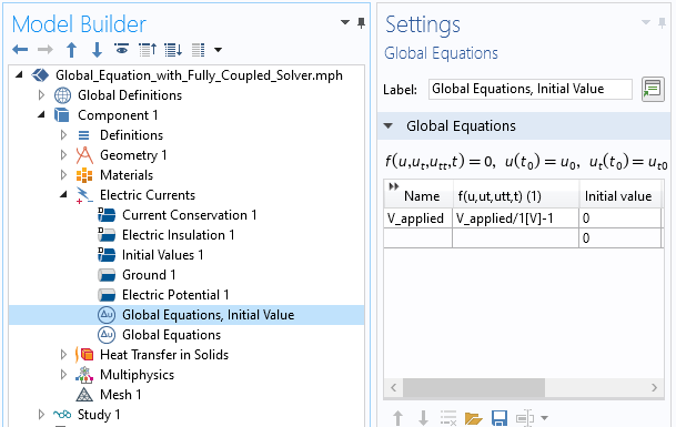
全局方程 设置,用于与 电流 接口 方程耦合的代数方程。
COMSOL 博客中有许多文章都对物理场的场变量与一个或多个常微分方程的耦合进行过介绍,包括:
此外,您还应该了解状态变量的相关主题。有关此主题的详细信息,请参阅博客文章:如何使用 COMSOL Multiphysics® 中的状态变量特征。
在创建方程之间的自定义耦合时,需要考虑一些重要的符号因素。在 COMSOL Multiphysics 中,作用在系统上的外部(广义)力应以正号进入方程,意味着质量-弹簧-阻尼方程在与其他方程耦合时,最好写作:


只要使用常微分方程建模,这种符号约定并不重要。但是,如果您使用 固体力学 接口将其与固体耦合时,则会有影响。这样的模型可以用于将质量黏在弹性物体的表面上。如果使用  的符号约定,则可以使用简单的双向约束进行耦合。如果使用
  ,则需要转换约束力表达式中的符号。在后一种情况下,耦合系统的对称性将被破坏,最终方程系统的非对称系统矩阵将降低求解效率。
洛伦兹方程系统
20 世纪 60 年代初,洛伦兹方程组被用于模拟大气对流。洛伦兹发现,在某些参数值和初始条件下,解呈现出混沌行为。如下图所示,在相空间中绘制的解类似于 “八字形”。洛伦兹吸引子是洛伦兹系统在相空间中的一组混沌解,关于使用 COMSOL Multiphysics 实现该系统的详细文档可在 此处 下载。
洛伦兹系统是非线性的,可以写成下面的形式


初始条件:


式中,参数 a、b 和 c 通常是正标量。并非所有解都是混沌的,但洛伦兹发现,a = 10、b = 8/3 和 c = 28 的值会产生一个具有混沌行为的方程组。下面的设置显示了具有以下初始条件的洛伦兹方程组:
u= −10v= −4.45w= 35.1
参数 pert 用于说明方程组对初始条件微小变化的敏感性。
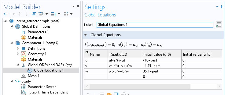
在 全局方程 接口输入的洛伦兹方程组。
下图显示了 0 s 到 35 s 之间的解:
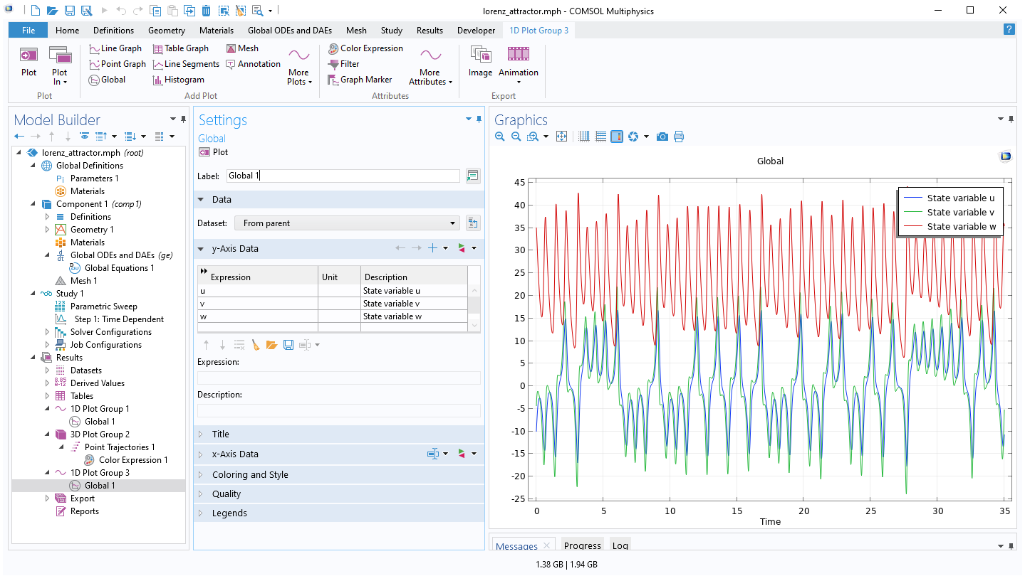 The Model Builder with the Global plot selected, the plot settings, and the Graphics window showing the state variable u in blue, the state variable v in green, and the state variable w in red.
洛伦兹方程组的解。
三维相空间的解显示了洛伦兹吸引子的特征形状。
 The Lorenz attractor with the outer section being red, the middle section being yellow, and the inner section being green.
洛伦兹方程组的相图,显示洛伦兹吸引子的特征形状。
在本文提供的可下载文件中,您还可以找到范德波尔振荡器的三维空间相图,其中以时间(刻度)为第三轴,绘制了类似的空间相图:
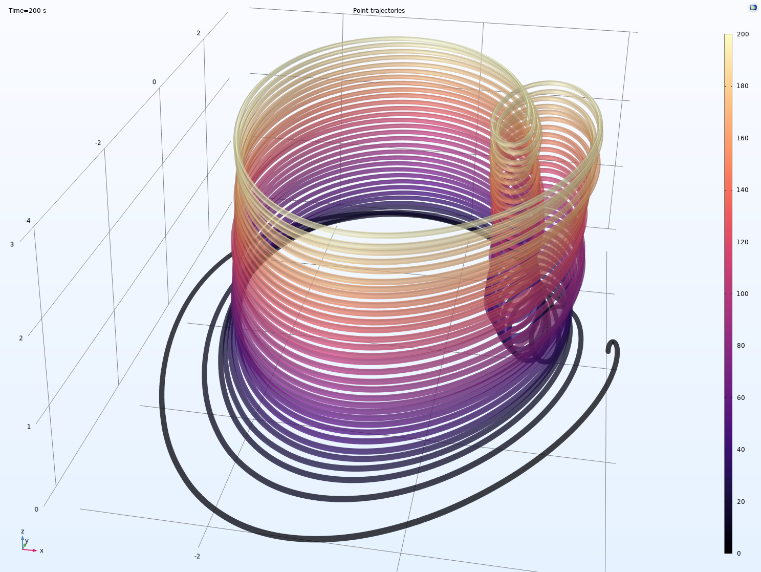 A 3D phase-space plot showing the shape in mostly purple and red, with black near the bottom and yellow near the top.
范德波尔振荡器方程解的三维空间相图。
进阶学习
虽然本文使用的模型可供下载,但我们鼓励您根据文中提供的指导建立自己的模型,这将有助于您巩固如何使用 全局常微分和微分代数方程 接口在软件中设置 常微分方程。
请提交与此页面相关的反馈,或点击此处联系技术支持。