
Diffusion Length and Timescales
Reaching Steady State in a Chemical System
Chemical systems involving diffusion often exhibit steady states where the concentration profile does not change as a function of time. For example, for material in a closed (impermeable) box, the steady-state concentration profile is the equilibrium where the concentration is constant everywhere. In the presence of any concentration gradient, diffusion will proceed to move mass from regions of high concentration to low concentration until a steady state is recovered. The mechanism of this process is discussed here. The concentration changes for an evolving system can be predicted by solving a diffusion equation.
When a chemical system is perturbed — resulting from, for example, a chemical reaction introducing a new flux of material into the system — diffusion will respond to restore the concentration profile to its new equilibrium. The time required for the recovery of a steady state is the diffusion timescale of the system. Until the steady state is reached, the influence of the perturbation will be felt only over a certain diffusion length scale. This length scale corresponds to the size of a diffusion layer (or sometimes, a depletion layer) in which the concentration has been altered from its initial condition.
Figure 1 illustrates the time variation of the concentration profile upon application of an elevated concentration to one surface of a system, where mass is removed at another surface. Diffusion is required to transport mass from the source to the sink. Consequently, the concentration at the surface evolves as time passes until a steady state is reached.
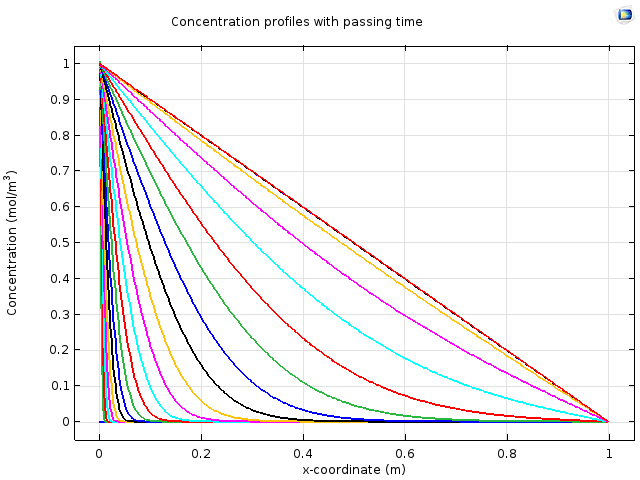
Figure 1: Concentration profiles on perturbing a 1D diffusion system.
Figure 1: Concentration profiles on perturbing a 1D diffusion system.
The concentration profiles are plotted for passing time following the application of an elevated concentration at the left of a one-dimensional geometry. The diffusion layer advances from left to right as time passes. At the final time (red line in Figure 1), the concentration gradient is constant, which also means that the mass flux is constant from the inlet to the outlet, yielding no accumulation of mass. Hence, the system is at a steady state where the concentrations no longer evolve in time.
Deriving Diffusion Length and Timescales
The simplest route to understanding the length and timescales of diffusion arises from dimensional analysis of the diffusion equation and diffusion coefficient. Recall the linear form of Fick's second law (the diffusion equation) for a single diffusing species:

Note that the equation relates the first time derivative to the second space derivative and that the diffusion coefficient has units of m2s-1. According to these dimensions, we can infer a relationship between the spatial and temporal extent of diffusion:

That is, the extent of a diffusion layer advances proportionally to the square root of elapsed time. Equivalently, the time required to reach steady state depends on the square of the length scale over which diffusion must take place. This proportionality is sometimes called the Einstein relation, with reference to the work of Albert Einstein that connected the statistics of diffusion with the macroscopic evolution of concentration through space and time.
Similarly, let us consider the nondimensionalization of the diffusion equation by introducing a reference timescale,  , and a reference length scale,
  . Then, for dimensionless time
  ,
,

Here, the dimensionless coefficient

is called the Fourier number. At a large Fourier number, the nondimensionalized time derivative is small — the concentrations approach a steady state that satisfies the steady-state diffusion equation. At a small Fourier number, the nondimensionalized time derivative is large — the concentrations remain far from a steady state and will continue to evolve in time.
While this approach of conceptual dimensional analysis is valuable, it is useful to check both the analytical and numerical solutions of the diffusion equation in order to confirm these relations. We can consider a simple example. Let us imagine a 1D space of extent L, which initially contains a reactant at a uniform concentration c0. At t = 0, the left-hand boundary changes its properties, such that a fast chemical reaction that consumes the species in question takes place. Therefore, the concentration at x = 0 will rapidly become zero. This type of system might be encountered in cases where there is a reaction of a biological component at a substrate or an electrochemical reaction at a large planar electrode.
How does the system respond? What is the overall rate of reaction? How long does it take before all of the mass is consumed? To answer these questions, we can perform a numerical simulation and solve the diffusion equation. Figure 2 shows a series of concentration profiles through elapsing time. Figure 3 shows the reaction flux, while Figure 4 shows the cumulative mass content of the system as time passes.
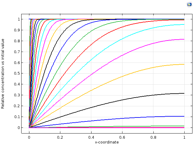
Figure 2: Concentration profiles measured versus the initial concentration of a chemical species that is rapidly consumed at the left of a box of finite length.
Figure 2: Concentration profiles measured versus the initial concentration of a chemical species that is rapidly consumed at the left of a box of finite length.
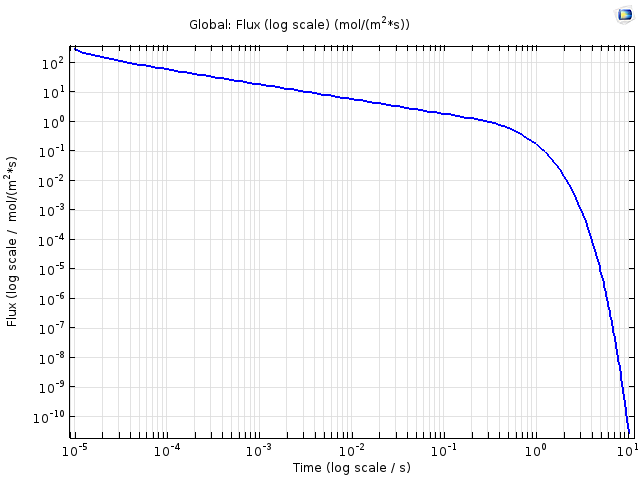
Figure 3: A log–log plot of the flux of material at the left of a diffusing system of finite extent.
Figure 3: A log–log plot of the flux of material at the left of a diffusing system of finite extent.
From Figure 3, we can identify that the dynamic behavior of the diffusion system transitions between two regimes. In the first regime, the advancing diffusion layer has not yet reached the right-hand side of the finite box; this will be the case at time frames short enough that the Fourier number is small. After the diffusion layer encounters the impermeable wall at the right-hand side of the box, the flux begins to fall more rapidly, and the mass content of the system depletes. At longer times, where the Fourier number is large, the new steady state (zero concentration everywhere) is attained.
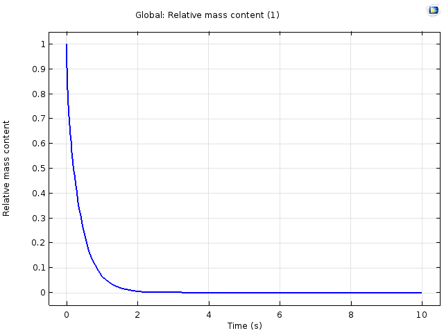
Figure 4: The evolution of total mass content (relative scale) for a system where material is lost by diffusion.
Figure 4: The evolution of total mass content (relative scale) for a system where material is lost by diffusion.
What about the case where an infinite amount of material is available for reaction? In this case, the concentration will never deplete in bulk. Instead, the diffusion layer continues to advance across a distance proportional to the square root of elapsed time, while the reaction rate will decrease according to the same proportion. This is the Cottrell problem, and it gives a well-known analytical solution:

The function  is the error function, which appears frequently in diffusional analysis. Here, note the recurring presence of the Einstein relation,

Differentiating the predicted concentration profile to find the diffusive flux at x = 0 yields a proportionality of the flux that leaves the system with  , which is confirmed by the gradient of -½ in the first part of Figure 3.
Using Diffusion Length and Timescales in Numerical Simulation and Modeling
Whenever a time-dependent problem is considered in which an equilibrium is perturbed and a system responds by diffusion, it is good practice to begin by evaluating the diffusion length and timescales. These can indicate whether a stationary or time-dependent analysis is required.
If the diffusion timescale is much shorter than the timescale of interest in the analysis of the system, then a stationary or quasistatic approach can be used. Alternatively, if the diffusion timescale is much longer than the timescale of interest, we can be sure that equilibrium is not attained. In this case, the diffusion length scale can be used to guide the required mesh density close to a boundary where material is added or removed in order to resolve the diffusion layer on the chosen timescale.
Published: April 24, 2023References
- A. Einstein, Annalen der Physik, vol. 17, pp. 549–560, 1905.
- F.G. Cottrell, Zeitschrift für Physikalische Chemie, vol. 42, pp. 385, 1903.