

在之前的博客文章中,我们讨论了近轴高斯光束公式。今天,我们将讨论更精确的高斯光束公式,COMSOL® 软件从5.3a 版本开始提供此公式。这种基于平面波展开的公式可以比传统的近轴公式更精确地处理非近轴高斯光束。
高斯光束的近轴性
众所周知的高斯光束公式仅适用于近轴高斯光束。近轴意味着光束主要沿光轴传播。有几篇论文从量化的角度讨论了近轴性(见参考文献 1)。
大体来说,如果束腰尺寸接近波长,则光束以更大的角度传播到焦点。因此,近轴假设行不通,公式不再准确。为了缓解这个问题,并提供一个更通用、更精确的高斯光束公式,我们引入了一个非近轴高斯光束公式。在用户界面中,这个公式称为平面波展开。
该方法基于平面波的角谱(参考文献 2),有时也称为角谱法(参考文献 3)。
平面波的角谱
我们简要回顾一下二维中的近轴高斯光束公式(为了获得更好的视觉效果和理解)。
我们先采用假设时谐场的麦克斯韦方程组,从中得到以下亥姆霍兹方程,用于波长为 \lambda 的偏振选择为面外的电场:
\left ( \frac
{\partial^2}{\partial x^2} +\frac{\partial^2} {\partial y^2}
+ k^2 \right ) E_z = 0,
其中 k=2 \pi/\lambda.
平面波的角谱基于以下这个简单事实:满足上述亥姆霍兹方程的任意场 可表示为以下平面波展开:
E_z(x,y) = \int_
{k_x^2+k_y^2=k^2}
A(k_y)e^
{i(k_x x +k_y y)}
dk_y,
其中 A(k_y) 是任意函数。
对于实数 k_x 和 k_y,积分路径是一个半径为 k 的圆。(对于复数 k_x 和 k_y,积分域延伸到复平面。)函数 A(k_y) 称为角谱函数。我们可以通过直接替换证明 E_z 满足亥姆霍兹方程。
既然我们知道这个公式总能给出亥姆霍兹方程的精确解,那么我们试着直观地理解它。根据约束k_x^2+k_y^2=k^2,我们可以设置 k_x=k cos(\varphi) 和k_y=k sin(\varphi) ,并将上面的公式重写为:
E_z(x,y) = \int_{-\pi/2}^
{\pi/2} A(\varphi)e^{ik(x \cos \varphi +y \sin \varphi)}d \varphi.
上述公式的含义是,它将波构造为向不同方向传播的许多波组成的和或积分,所有波都具有相同的波数k,如下图所示。
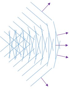
平面波角谱的可视化效果。
回到k_y的表示形式,当实际上使用此公式解决问题时,您要做的就是找到角谱函数A(k_y) 以满足边界条件。 通过假设横向场的轮廓(垂直于传播方向,即光轴)也是高斯形状(请参见Ref. 4),可以推导A(k_y) = \exp(-k_y^2 / w_0^2) ,其中w_0是频谱宽度 。
通过更多的数学操作,我们得到了光谱宽度和束腰半径之间的关系。 例如,对于慢速高斯光束,其角谱很窄。 另一方面,平面波是极端情况,其中角谱函数是增量函数。 对于快速的高斯光束,角谱较宽,反之亦然。
这是非近轴高斯光束基础理论的简要概括。为了回顾到目前为止我们所展示的内容,我们使用极坐标再次重写公式 x=r \cos \theta, \ y = r \sin \theta:
A(\varphi) e^
{ikr \cos (\theta-\varphi)}
d \varphi.
这是 Born 和 Wolf(参考文献 2)在他们的书中使用的表述。
三维公式较为复杂,由于发生偏振,看起来有所不同,但基本思想与上述参考文献中的相同。根据你是否考虑倏逝波,它也可能有所不同。波动光学模块和 RF 模块中使用的平面波展开方法虽然基于角谱理论,但适用于数值计算。
平面波展开:设置和结果
我们将新特征平面波展开 与之前的特征近轴近似 进行比较。包含这两种方法的设置 窗口如下所示。
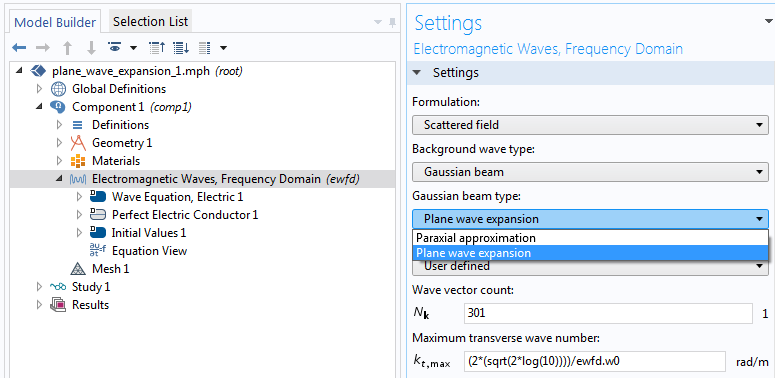
平面波展开特征设置。
使用新特征情况下,如果自动 设置无法给出令人满意的近似值,有两个选项可以选择:
- 波矢数
- 最大横波数
第一个选项决定离散化级别的数量,具体取决于你想要表示高斯光束的精细程度。平面波越多,越精细。第二个选项与前一个方程中的积分界限有关;即 -\pi/2 \le \varphi \le \pi/2。根据高斯光束的速度,对于可能的最小光斑尺寸,积分界限可以是最大值 \pi/2,对于较慢的光束,积分界限可以更浅。你需要更多有角度的平面波和更大的横波数来表示更快(更集中)的光束。
以下结果比较了光斑半径为 \lambda/2的两个公式,该半径为非近轴性。与上一篇博客文章一样,仿真是用散射场 公式完成的,并且域由完美匹配层(PML)包围。这样,散射场表示精确亥姆霍兹解的误差。
下面的左图显示了新特征,右图显示了近轴近似。顶部图像显示了计算的高斯光束背景场的模 ewfd.Ebz,底部图像显示散射场模 ewfd.relEz,它表示精确亥姆霍兹解的误差。显然,在非近轴方法中,亥姆霍兹解的误差大大减小。

平面波角谱与近轴公式的比较。
结束语
我们讨论了用新的平面波展开方案近似非近轴高斯光束的理论和结果。这个公式非常精确,但在假设条件下仍然是近似值。首先,我们假设焦平面中的场形状。其次,我们假设倏逝场为零。如果关注快速高斯光束聚焦区附近的某些纳米结构的场耦合,你可能需要计算倏逝场。
后续操作
单击下面的按钮,了解更多关于 COMSOL® 软件中用于大规模光学问题建模的公式和特征:
注:此功能也可以在 RF 模块中找到。
参考文献
- P. Vaveliuk, “Limits of the paraxial approximation in laser beams”, Optics Letters, vol. 32, no. 8, 2007.
- M. Born and E. Wolf, Principles of Optics, ed. 7, Cambridge University Press, 1999.
- J. W. Goodman, Fourier Optics.
- G. P. Agrawal and M. Lax, “Free-space wave propagation beyond the paraxial approximation”, Phys. Rev. a. 27, pp. 1693–1695, 1983.

评论 (19)
妙 彭
2020-03-11Thanks Yosuke for such detailed explanation. The model I am currently working on is a Gaussian beam focused by a high NA (=1.25) objective lens. But I don’t know how to produce the tightly focused Gaussian beam with comsol. Can you help me ?
wei bao
2020-03-12 COMSOL 员工如果你能写出这个高斯波的表达式,那可以直接在COMSOL中用自定义表达式来输入
妙 彭
2020-03-13谢谢您的解答!我在文献调研中,发现可以利用Richards-Wolf矢量衍射理论计算高NA值透镜附近的入射场。而博客中提到的以角谱法为基础,对高斯光束进行平面波展开的求解方法,也是采用该衍射理论进行分析的。并且博客中还提到,“你需要更多有角度的平面波和更大的横波数来表示更快(更集中)的光束”。所以我的第一直觉是,可以通过设置高斯波类型为“平面波展开”,随后在“用户定义”中增加“最大横波数”和“波矢数”,即可得到紧聚焦高斯光束。但是采用这种方式进行仿真分析,发现得不到紧聚焦的高斯光束。所以按照您的说法,我是首先需要根据Richards-Wolf矢量衍射理论计算出经过高NA值透镜之后的电场分布,随后在用户自定义表达式中输入,那么在这种情况下,我是否还需要设置高斯光束类型为”平面波展开“,是否还需要增加”最大横波数“和”波矢数“呢?
wei bao
2020-03-13 COMSOL 员工这种情况下,您可以直接使用自定义表达式,不需要设置为平面波展开了
妙 彭
2020-03-13好的,谢谢您的解答!不过我还有一个疑问:高斯光束类型设置为“平面波展开”,不能直接用于设置紧聚焦的高斯光束吗?
Yosuke Mizuyama
2020-03-13 COMSOL 员工Hi,
Thank you for reading my blog.
Are you talking about the liquid immersion lens?
If so, it’s a little bit tricky to set it up correctly.
1. Calculate the NA in the vacuum instead of your material. NA_vac = 1.25/n. (I assume your liquid’s index is 1.51 or something. Then the NA_vac is about 0.83.)
2. Calculate a rough spot radius from the above result, r = 0.61*lambda/NA_vac (= 0.73*lambda if n=1.51).
3. From the above calculation, determine if your beam is paraxial or non-paraxial. If it’s a liquid immersion lens, it is most likely highly non-paraxial. So you will have to use the non-paraxial Gaussian beam option with the plane wave expansion.
4. In a liquid, Gaussian beams change the focal position. You will have to calculate the focal position shift in your liquid. Probably you will have to use the Gaussian ABCD method. Refer to Shojiro Nemoto, “Waist shift of a Gaussian beam by plane dielectric interfaces”, Applied Optics, Vol. 27, No. 9 (1988) for this focus shift physics.
5. Back-calculate the focal position in the vacuum and enter the focal position in the “Beam radius” setting in COMSOL.
Since your beam is highly non-paraxial, you will need more settings.
6. Select Plane wave expansion
7. Select User defined for Wave vector distribution type
8. Enter a certain large number for Wave vector count, say 40.
9. Enter a certain number larger than ewfd.k0, say 1.2*ewfd.k0
10. Enter the beam radius you calculated above
11. Enter the adjusted focal position in the vacuum that you calculated above
Then it should work.
This is a highly difficult and advanced simulation. You may need to contact support@comsol.com for your successful settings of this since there is limitation for teaching in this comment space.
Best regards,
Yosuke
妙 彭
2020-03-14Hi, Dr. Yosuke,
Thank you very much for your kindness help and patience. But I still have some confusion and need your help.
1. Yes, I am talking about the liquid immersion lens, and the liquid’s index is 1.51.
2. If the focus position is in water (n = 1.33) rather than in vacuum or air, do I need to consider the refractive index of water according to the formula you provided: r = 0.61*lambda/NA_vac?
3. As you mentioned in point 5, should it be enter the spot radius in the “Beam radius”, and the focal position in the “focal plane along the axis” in COMSOL?
4. As you mentioned in point 8 and 9, How to calculate the wave vector count and the maximum transverse wave number? Can I set any number I want? And iust make sure that this number is greater than ewfd.k0?
5. Actually, I am trying to simulate the motion of nanosphere in an optical tweezer system using COMSOL. After the Gaussian beam passes through the oil-immersed objective lens (NA = 1.25), it will illuminate on the nanospheres, where the environment is water (n = 1.33), and then focus behind the nanospheres. So, when I calculate the focal position, whether the refractive index of microsphere and water should be considered? And when the position of the microsphere changes, does the focal position need to be recalculated every time?
I am very sorry to bothering you again, but I sincerely hope to receive your reply.
Best wishes
Miao Peng
Yosuke Mizuyama
2020-03-15 COMSOL 员工Hi Miao,
Some of your questions are difficult to answer here and probably only you know the answer. Please contact COMSOL support with your model file.
The settings for the wave vector count and the max transverse wave number are not something that can be uniquely calculated. It’s a trade-off between the accuracy and the aliasing issue. So you will have to tweak it around. But please try 40 and 1.2*ewfd.k0 as I mentioned as starting points.
Once you have fixed the focal position for the initial nanosphere position, you don’t have to change it even if the sphere moves around unless the beam moves around as well.
I hope this helps.
Best regards,
Yosuke
妙 彭
2020-03-15Hi, Dr. Yosuke,
Thank you very much for your detailed explanation. It will help me a lot. And I am looking forward to more such a brilliant blogs in the future, maybe more about the simulation of optical tweezers.
Best wishes
Miao Peng
Yosuke Mizuyama
2020-03-17 COMSOL 员工You are welcome!
Best regards,
Yosuke
妙 彭
2020-03-19Hi,Dr. Yosuke
I am sorry to bothering you again.
But I still have doubts about your solution last time.
1. In COMSOL 5.5, does the plane wave expansion formula of Gaussian beam is transmitted in vacuum by default? So when we think about transmission in other media, we need to consider the refractive index of the media, right?
2. You said, “Calculate a rough spot radius from the above result, r = 0.61*lambda/NA_vac.” If my focus is in a medium such as water or air, do I need to consider the effect of the refractive index of the medium on the spot size?
3. In “ewfd” setting, the default value of the “Focal plane along the axis” of the beam is zero, right? If so, when the focus position of the tightly focused Gaussian beam is in the water, is the calculated “focal position shift” should be directly enter in the text box of “Focal plane along the axis”?
I am very sorry to take up your precious time to answer for me again. I am looking forward to your reply.
Best wishes
Sincerely,
Miao Peng
Yosuke Mizuyama
2020-03-19 COMSOL 员工Hi Miao,
I think you have to consider if the background field feature is appropriate or not for your application. We’ve been discussing under an assumption that you can somehow use the background field formulation by doing some pre-calculations. But it may be more appropriate to use the Gaussian beam boundary condition, rather than the (domain) background. We introduced the Gaussian beam feature in the scattering boundary condition at version 5.5 but it’s only the paraxial formulation. For your high NA case, you can use the integral formula that I wrote in this blog.
Best regards,
Yosuke
妙 彭
2020-03-24Hi, Dr. Yosuke
Thank you for your kindness help again. I see what you mean.
Best wishes
Sincerely,
Miao Peng
meijie li
2024-11-14您好,请问如何在一个简单的二维真空板中激发一个复频率的倏逝波
子奇 陈
2024-11-19 COMSOL 员工可以尝试:1.背景场公式,例如平面波乘上虚部的幅值衰减因子;2.边界模式分析,选择那些具有合适虚部的结果,或者已知端口的分布以及相应的复传播系数,然后在用户定义端口中设定。
盛 杨
2024-12-25你好,这两个对比的模型,有么?是否可以发一份给我,谢谢
子奇 陈
2024-12-31 COMSOL 员工你好,目前暂时没有模型可以提供。
盛 杨
2024-12-26你好,有这两个对比模型的具体设置参数么?我这边设置参数,当焦斑直径小于波长,焦点位置只在边界
子奇 陈
2024-12-31 COMSOL 员工对于紧聚焦高斯光束,如果考虑纵向成分,也就是计算倏逝场,在最大横波数中,设置为大于ewfd.k0的时候,目前对这种光束汇聚空间,或者说是相对传播方向的负空间没有很好的数值定义,所以仅能够对正空间部分,也就是发散的正空间进行仿真。所以焦点只能在边界。如果是不考虑倏逝成分,则可以焦点设置在场内,但此时有一定的误差。详细信息可以阅读该作者的其余相关文章。